Geometric Design and Railway Alignment
Table of Contents
Chapter I Generalities
I.1 Centrifugal Force:
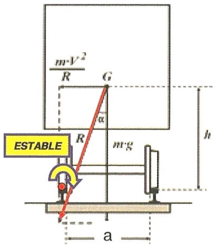
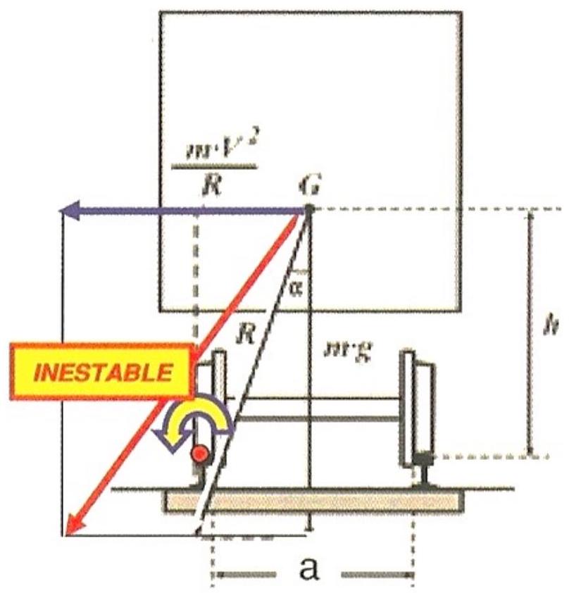
When a railway composition transitions from a straight segment to a curved trajectory, it experiences the action of a transverse force known as centrifugal force ( \(\boldsymbol{F}_{\mathbf{c}}\) ), whose magnitude is expressed by the following fundamental relation.
\[F_{c}=m \cdot \alpha_{c}=\frac{m \cdot V^{2}}{R} \quad \text { where: } \quad \alpha_{c}=\frac{V^{2}}{R}\]In this mathematical formulation, the variable m represents the total mass of the train, V designates the instantaneous displacement velocity, and R corresponds to the value of the radius of curvature of the circular geometric element. The centrifugal acceleration \(\left(\alpha_{c}\right)\) constitutes a determining parameter that allows quantifying the intensity of the transverse dynamic effect.
From a practical perspective, when a composition moves at 100 km/h through a curve whose radius of curvature is 350 meters, the resulting centrifugal acceleration reaches approximately 2.2 m/s². Considering the comfort criteria established in railway engineering, the maximum acceleration value that a traveler can tolerate without experiencing significant discomfort is around 1 m/s².
To mitigate the detrimental effects of this uncompensated acceleration, the technical solution contemplates the strategic implementation of track cant (superelevation) and the incorporation of transition curves that allow for a gradual variation of curvature.
I.2 Centrifugal Acceleration
When a railway composition travels along a curved path under the influence of uncompensated accelerations, a series of adverse effects are generated on multiple components of the railway system.
Regarding the dynamic behavior of rolling stock, the presence of uncompensated transverse accelerations causes the generation of considerable dynamic forces at the wheel-rail interfaces, especially at the entry and exit tangent points of curved elements. These forces, combined with the oscillatory phenomena inherent to the movement of rolling stock, can, under certain high-speed circumstances, originate instability situations that can potentially lead to derailment phenomena or even overturning of the composition. Additionally, the excessive demand imposed on vehicle suspension systems generates significant increases in maintenance and conservation costs.
The railway infrastructure also experiences detrimental effects derived from these uncompensated accelerations. A pattern of differential wear occurs between both rail heads, with greater intensity on the outer rail of the curve. Transverse degradation phenomena of the track structure appear, along with an increase in the workload of fastening systems and a tendency for the rail located on the outside of the curve to overturn.
From the perspective of the rail transport user, these effects generate direct negative consequences such as feelings of discomfort, dizziness, and the perception of unpleasant lateral movements. In freight transport contexts, these phenomena can cause the unwanted displacement of transported goods inside cargo vehicles.
To neutralize these unfavorable effects on operational safety and user comfort, a geometric strategy is implemented consisting of progressively elevating the rail located on the outside of the curve with respect to the inner rail. This transverse inclination of the platform generates a reorientation of the resultant forces acting on the vehicle’s mass, producing its alignment with respect to the perpendicular to the track plane. As a consequence of this geometric configuration, the disturbing lateral acceleration effectively disappears, simultaneously improving safety conditions and circulation comfort.
Chapter II Cant (Superelevation)
The implementation of cant in railway track geometry constitutes a fundamental design variable that can be quantified and expressed through two alternative methodological approaches, each with its particularities and specific applications in distinct operational contexts. The first approach defines superelevation, that is, the vertical height difference existing between the head of the rail located on the inside of the curve and the head of the rail located on the outside. This magnitude is usually measured in millimeters and constitutes the traditional methodology historically used in Spain. The adoption of this criterion presents certain operational limitations, since it requires the definition of differentiated values for maximum superelevation, cant deficiency, and cant excess specifically as a function of the available track gauge. In contexts where a third rail is implemented to allow the circulation of compositions with two different track gauges, this methodology forces the establishment of two differentiated superelevation values for each gauge, which complicates operational design. When cross-section increases (gauge widening) are incorporated in certain sections to improve curve geometry, it is necessary to proportionally increase the superelevation value to maintain the transverse inclination that effectively compensates for the centrifugal force. In these situations, admissible cant values will be lower than those used without gauge widening, particularly in small radius curved tracks that demand maximum cant. From a technical documentation and graphic representation perspective, superelevation always adopts a positive numerical value, so it is necessary to incorporate additional information in lists and diagrams to explicitly indicate the direction of the track inclination.
The second approach describes cant through transverse inclination expressed as a percentage. This criterion presents the significant advantage of being independent of the specific track gauge, allowing the application of unified criteria for deficiency, excess, and maximum cant value regardless of the track gauge being worked with. The sign assignment to cant follows orientation criteria: it is considered positive when the curvature radius is positive, that is, when the curve develops to the right in the direction of travel; it will be negative in the opposite case. From a comparative technical perspective, the Spanish approach based on superelevations presents disadvantages in criteria coherence, so the adoption of transverse inclination as a fundamental variable would constitute a significant improvement. However, the need to maintain homogeneity with current international standards, where the use of superelevations predominates, limits the implementation of this methodological change.
In terms of practical track geometric configuration, when both rail heads are located on the same horizontal plane, the centrifugal force would act to push the composition towards the outside of the curve, causing a heterogeneous distribution of loads between both rail heads. This situation would generate conditions of derailment risk, unstable rolling movement, lateral accelerations of considerable magnitude, and significant deficiencies in comfort levels for passengers and cargo. The technical solution contemplates the inclination of the track plane towards the inside of the curve, modifying the orientation of the resultant forces acting on the vehicle mass. This resultant should ideally be located as close as possible to the longitudinal axis of the track, always maintaining its point of application between the wheel support areas. This configuration allows the reaction of the outer rail to resist the potential overturning moment.
Ferrocarriles metropolitanos: tranvías, metros ligeros y metros convencionales. Manuel Melis
II.1 Theoretical Cant
Cant is operationally defined as the vertical level difference \(\boldsymbol{z}\) between the two rail heads, this height difference being measured in a section perpendicular to the track axis. When a cant value is implemented that fully compensates for the manifestation of the centrifugal force, the resultant \(\boldsymbol{R}\) of the composition of the centrifugal force \(\boldsymbol{F}_{\mathbf{c}}\) and the gravitational weight \(\boldsymbol{W}\) acquires a normal orientation with respect to the plane defined by the track. This specific configuration is designated as theoretical cant or ideal cant.
Through geometric and dynamic considerations, the relationship between the tangent of the track plane inclination angle can be established: \(\tan \alpha=\frac{F_{c}}{W}=\frac{m \cdot \frac{V^{2}}{R}}{m \cdot g}=\frac{V^{2}}{g \cdot R}\)
Simultaneously, the cant geometry allows expressing:
\[\sin \alpha=\frac{z}{a} \rightarrow \tan \alpha=\frac{z}{\sqrt{a^{2}-z^{2}}}\]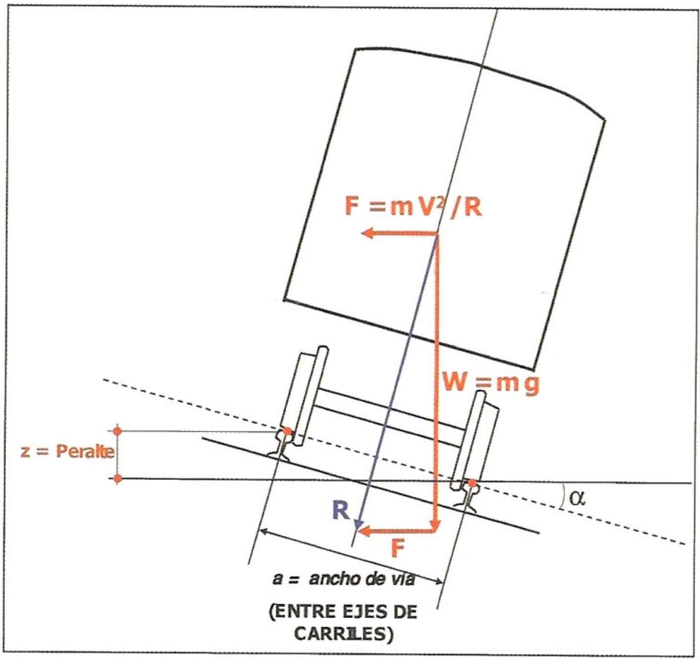
Ferrocarriles metropolitanos: tranvías, metros ligeros y metros convencionales. Manuel Melis
In Spanish railway systems under RENFE administration, operating with UIC 60 rails that have a head width of 72 millimeters, the track gauge turns out to be:
\[a=1.668+0.072=1.740 \mathrm{~m}\]For metro-type urban transport systems with a track gauge of 1.445 meters and using UIC 54 rails with a head width of 70 millimeters:
\[a=1.445+0.070=1.515 m\]Establishing the equality between the two expressions derived from the analysis of the force polygon and the cant geometry, the mathematical expression is obtained that provides the exact value of the cant required by a composition circulating at velocity V on a curved trajectory of radius R to completely annul the manifestation of centrifugal force:
\[\frac{V^{2}}{g \cdot R}=\frac{z}{\sqrt{a^{2}-z^{2}}} \rightarrow z=\frac{a \cdot V^{2}}{\sqrt{g^{2} \cdot R^{2}+V^{4}}}\]To illustrate the practical application of these fundamental relationships, let us consider the specific case of a high-speed train (AVE) circulating at the nominal speed of 300 km/h (equivalent to 83.3 m/s), traversing a curved trajectory whose radius of curvature is 7000 meters. Using the standard international track gauge of 1.435 meters plus the rail width of 0.072 meters, the necessary theoretical cant turns out to be:
\[z=\frac{a \cdot V^{2}}{\sqrt{g^{2} \cdot R^{2}+V^{4}}}=\frac{1,507 \cdot(83,3)^{2}}{\sqrt{(9,8)^{2} \cdot 7000^{2}+(83,3)^{4}}}=0,1516 m\]The resulting transverse inclination angle is calculated by:
\[\sin \alpha=\frac{z}{a}=\frac{0,1516}{1,507}=0,1006 \rightarrow \alpha=5,77^{\circ}\]Historically, in previous developments of railway engineering, a simplifying approximation was made where the sine of the angle was assimilated to its tangent, which facilitated calculations before the computational era:
\[\sin \alpha \cong \tan \alpha=\frac{z}{a} \rightarrow \frac{z}{a}=\frac{V^{2}}{g \cdot R} \rightarrow z=\frac{a \cdot V^{2}}{g \cdot R} \rightarrow z_{t, \max }=\frac{a \cdot V_{\max }^{2}}{g \cdot R}\]From this approximation, the simplified mathematical expressions were derived that have been historically applied in Spain for practical calculation, the variables being expressed in units of: z in millimeters, a in meters, g in m/s², V in km/h, and R in meters:
\[\begin{gathered} \frac{z}{1000}=\frac{a}{g} \cdot\left(\frac{1000}{3600}\right)^{2} \cdot \frac{V^{2}}{R} \\ z=13.7 \cdot \frac{V^{2}}{R} \text { RENFE gauge } \quad(a=1.668+0.070) \\ z=11.8 \cdot \frac{V^{2}}{R} \text { UIC gauge } \quad(a=1.435+0.070) \end{gathered}\]II.2 Uncompensated Acceleration
Uncompensated acceleration varies depending on the specific circulation speed. This variability implies that certain railway compositions will experience an insufficiency in the magnitude of the implemented cant, while others will endure an excess of it. To illustrate this problem, consider a 1,000-meter radius curve developed on a RENFE gauge track with dimensions \((\mathrm{a}=1.668+0.072=1.740 \mathrm{~m})\):
| Composition Type | Speed | Required Cant |
|---|---|---|
| TALGO | 160 km/h | 350 mm |
| Freight Train | 80 km/h | 88 mm |
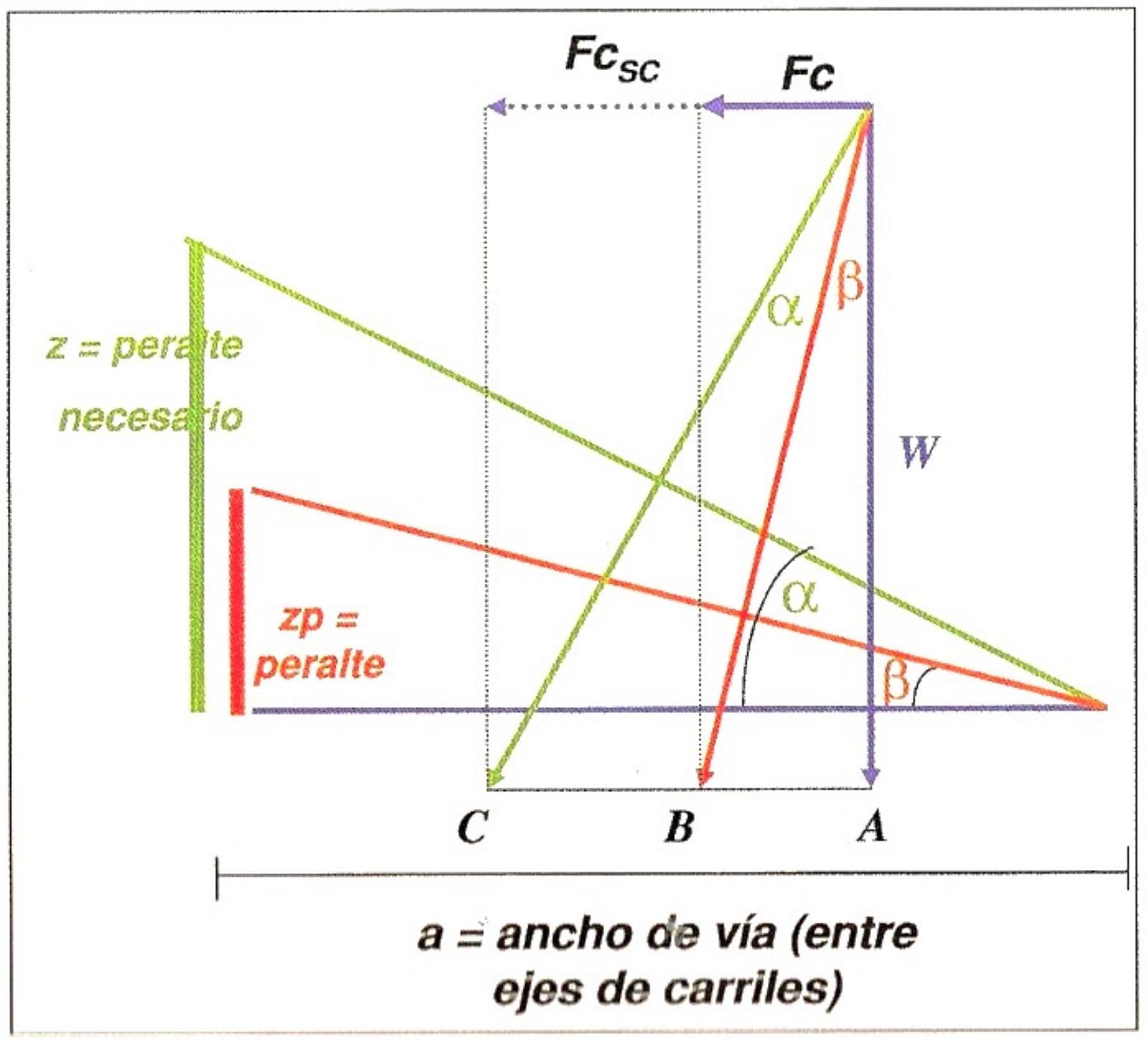
This heterogeneous situation highlights the need to implement a compromise cant that does not fully satisfy the requirements of any of the composition types but represents a balanced technical solution.
From the force analysis point of view, suppose a composition requires a cant angle \(\alpha\) (corresponding to a level difference z), but the track implements only an angle \(\beta\) (level difference \(\boldsymbol{z}_{\boldsymbol{p}}\)). In this analysis, the total centrifugal force is represented by segment AC, while the implemented cant compensates only a portion of said force, corresponding to segment AB which represents the partially compensated centrifugal force \((\mathbf{F}_{\mathbf{c}})\).
Ferrocarriles metropolitanos: tranvías, metros ligeros y metros convencionales. Manuel Melis
The centrifugal force that remains uncompensated is designated as \(\boldsymbol{F}_{\boldsymbol{c}, \mathbf{s c}}\) and corresponds to segment BC of the force diagram. Through vector analysis, we can establish the following relationships:
\[F_{c, S c}=B C=A C-A B=W \cdot \tan \alpha-W \cdot \tan \beta\]Expanding this expression in terms of fundamental physical parameters:
\[F_{c, s c}=W \cdot\left[\frac{F_{c}}{W}-\frac{z_{p}}{a}\right]=m \cdot g \cdot\left[\frac{m \cdot V^{2}}{m \cdot g \cdot R}-\frac{z_{p}}{a}\right]=m \cdot\left[\frac{V^{2}}{R}-\frac{g \cdot z_{p}}{a}\right]\]Consequently, the uncompensated acceleration \(\alpha_{s c}\) experienced by the composition can be expressed as:
\[\alpha_{s c}=\frac{V^{2}}{R}-\frac{g \cdot z_{p}}{a}\]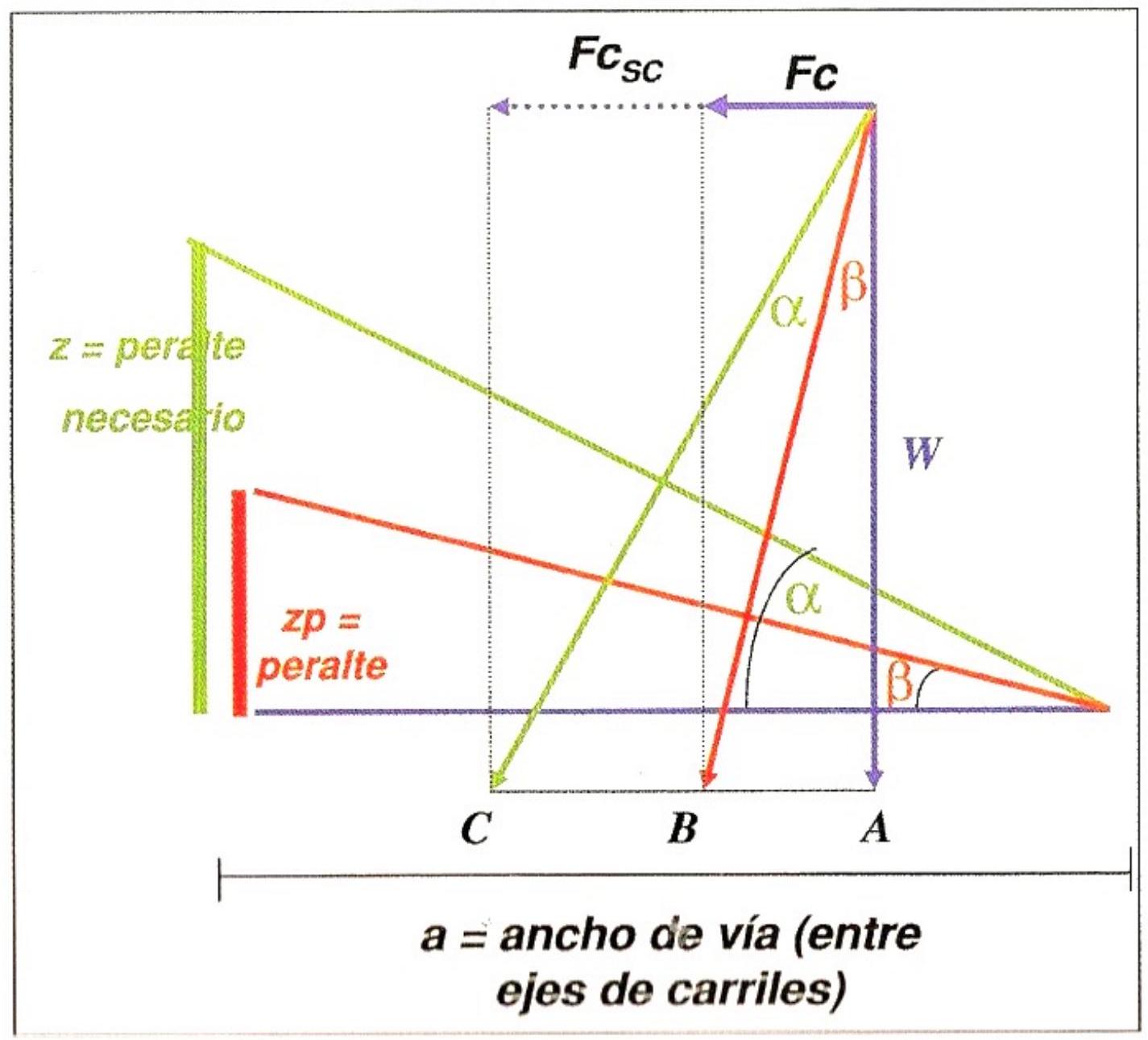
II.3 Cant Deficiency
When the track is provided with a cant \(\boldsymbol{z}_{\boldsymbol{p}}\) whose magnitude is insufficient to fully compensate for the action of the centrifugal force, cant deficiency (designated as I) is defined as the dimensional difference between the required theoretical cant z and the implemented cant \(\boldsymbol{z}_{\boldsymbol{p}}\).
Through geometric and dynamic considerations, we can establish that: \(\tan \alpha=\frac{F}{W}=\frac{m \cdot \frac{V^{2}}{R}}{m \cdot g}=\frac{V^{2}}{g \cdot R}\)
The geometry of the cant implemented with deficiency is expressed by: \(\sin \alpha=\frac{z_{p}+I}{a} \approx \tan \alpha\) (when \(\alpha\) is a small angle)
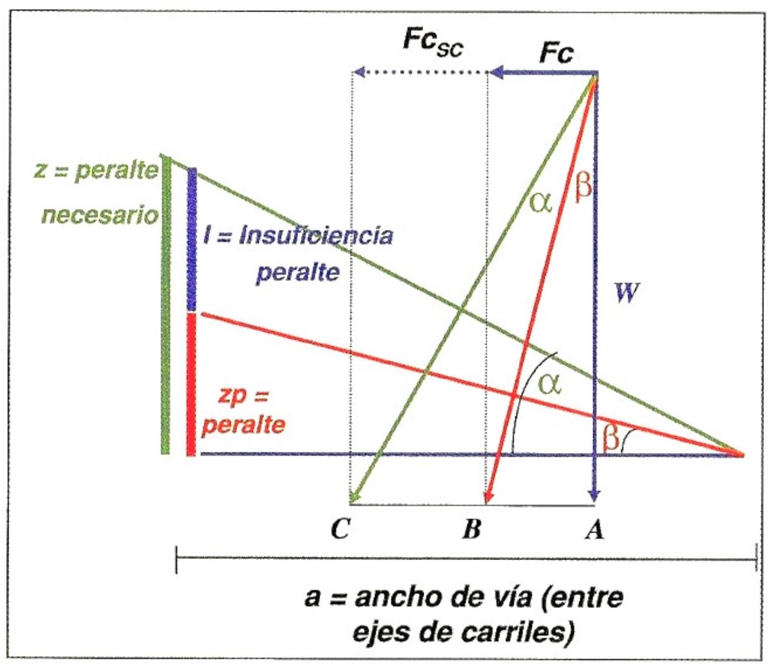
Equating both expressions for small angles, where the approximation \(\tan \alpha \approx \sin \alpha\) is valid:
\[\frac{z_{p}+I}{a} \approx \frac{V^{2}}{g \cdot R}\]Developing algebraically to obtain the value of cant deficiency:
\[I=\frac{a \cdot V^{2}}{g \cdot R}-z_{p}=z_{t, \max }-z_{p}\]Considering the fundamental relationship between uncompensated acceleration and cant deficiency:
\[\alpha_{s c}=\frac{V^{2}}{R}-\frac{g \cdot z_{p}}{a}\]Multiplying this expression by the quotient between the track gauge and gravity:
\[I=\alpha_{S C} \cdot \frac{a}{g}\]
II.4 Cant Excess
Contrary to the case of deficiency, when the implemented cant exceeds the value theoretically required for a specific circulation speed, the phenomenon is designated as cant excess and is denoted by the variable E. In this situation, E being the cant excess:
\[\frac{z-E}{a}=\frac{V^{2}}{g \cdot R}\]Cant excess generates an uncompensated transverse acceleration directed towards the inside of the curve, which is expressed by:
\[E=\frac{\alpha_{S C} \cdot a}{g}\]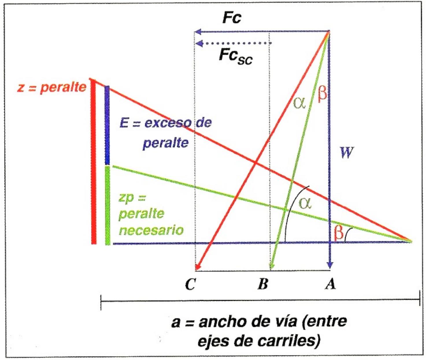
It is convenient to point out that in practical operational contexts, slow-moving compositions, particularly freight trains, constitute types of traffic for which it is not necessary to impose strict limitations on uncompensated acceleration, since passenger comfort does not constitute a determining consideration.
II.5 Practical Cant
II.5.1 Heterogeneous Traffic
When the railway infrastructure is subject to the circulation of multiple categories of compositions with heterogeneous operational characteristics, the design solution requires the adoption of a compromise cant that balances the conflicting requirements of the different types of traffic.
This compromise strategy must be based on deep technical considerations regarding the specific composition of the traffic operated on the line in question. The objective is to implement a cant that minimizes adverse effects both for the dynamic behavior of the compositions and for the integrity of the infrastructure, while simultaneously respecting the comfort and safety criteria of transport users.
In Spanish practice, the methodology traditionally applied has consisted of establishing the practical cant through the relationship:
\[z_{p}=\frac{2}{3} \cdot z_{t}\]There are various alternative methodological criteria to determine the compromise cant:
-
Direct implementation of the two-thirds criterion: \(z_{p}=\frac{2}{3} \cdot z_{t}\), which generates \(z=13.7 \cdot \frac{V_{\text {max }}^{2}}{R} \cdot \frac{2}{3} \approx 9 \cdot \frac{V_{\text {max }}^{2}}{R}\) for RENFE gauge and \(z=11.8 \cdot \frac{V_{\text {max }}^{2}}{R} \cdot \frac{2}{3} \approx 8 \cdot \frac{V_{\text {max }}^{2}}{R}\) for UIC gauge.
-
Cant calculation for a reduced speed: \(z_{p}\) determined for \(V=0.8 \cdot V_{\text {max }}\)
-
Use of a weighted average speed: \(z_{p}\) obtained for \(V=\sqrt{\frac{V_{\text {max }}^{2}+V_{\text {min }}^{2}}{2}}\)
-
Application of a weighted average speed by circulation frequency: \(V=\sqrt{\frac{\sum_{m} V_{m}^{2} \cdot N_{m}}{\sum_{m} N_{m}}}\)
Where \(V_{m}\) represents the characteristic circulation speed of each specific train category m, and \(N_{m}\) designates the number of compositions belonging to each category m that use the infrastructure during a reference period.
II.6 Limitations of Cant Values
In establishing the permissible limits for cant values that can be implemented on a railway line, it is observed that the most rigorous restrictions come from considerations related to the comfort of the passenger transport user. Fortunately, limitations derived from potential problems in vehicles or track infrastructure are less restrictive.
Regarding the classification of railway rolling stock, current regulations establish different categories characterized by the maximum admissible values of uncompensated transverse acceleration:
- “Normal” Type: Maximum acceleration of \(0.65 \mathrm{~m} / \mathrm{s}^{2}\) (designation without additional complement letter for maximum speed).
- Type A: Maximum acceleration of \(1 \mathrm{~m} / \mathrm{s}^{2}\).
- Type B: Maximum acceleration of \(1.2 \mathrm{~m} / \mathrm{s}^{2}\).
- Type C: Maximum acceleration of \(1.5 \mathrm{~m} / \mathrm{s}^{2}\).
- Type D: Maximum acceleration of \(1.8 \mathrm{~m} / \mathrm{s}^{2}\).
II.6.1 Fast Trains
Experimental research carried out in the field of railway engineering has consistently demonstrated that the fundamental limiting criterion is passenger comfort, being more restrictive than structural safety criteria limiting the potential overturning of rolling stock. When designs are implemented that fully respect passenger comfort standards, safety coefficients regarding overturning acquire considerably high values, typically in the range of 6 to 10.
The perception of comfort during circulation on curved trajectories is directly conditioned by the magnitude of the uncompensated acceleration experienced by the passenger.
To adequately evaluate the acceleration effectively supported by passengers, it is essential to consider the dynamic effects of the vehicle suspension system. The suspension system is specifically designed to attenuate the adverse effects of transient vibrations and random accelerations.
However, during circulation on curved trajectories, the suspension system introduces dynamic complications. The effect of transverse acceleration causes the compression of shock absorbers located on the outside of the curve, while simultaneously lengthening the shock absorbers on the inside. This differential deformation process significantly reduces the effectiveness of the implemented cant, generating an uncompensated acceleration that exceeds what should theoretically occur.
To mathematically quantify these suspension system flexibility effects, the parameter called “flexibility coefficient” designated as s is introduced. Current UIC regulations establish a maximum limit of \(\boldsymbol{s}=\mathbf{0.4}\) to classify vehicles with soft suspension. Historically, vehicles manufactured in previous periods presented values of this coefficient up to 0.6, and examples of these characteristics still circulate on numerous railway networks worldwide.
Modern design compositions, when operating at full load capacity, typically present a suspension flexibility coefficient in the order of 0.4.
Applying these principles to specific operation cases, representative values of cant deficiency can be determined that are tolerable according to the practices of different railway administrations. The general mathematical expression encompassing these criteria is:
\[\alpha_{s c} \cdot(1+s)=\frac{V^{2}}{R}-\frac{g \cdot z_{p}}{a} \cdot(1+s)<\alpha_{s c, \text { passenger }}\]ADIF technical regulations establish the following maximum limits for allowed uncompensated acceleration according to train category:
For compositions classified as Normal Trains, a maximum permissible uncompensated acceleration of \(\alpha_{s c} \mathbf{= 0.65} \boldsymbol{m/s^{2}}\) is specified.
For compositions classified as Type A Trains, a maximum permissible uncompensated acceleration of \(\mathbf{1.00 ~m/s^{2}}\) is specified.
For Type B Trains (pendular TALGO), the maximum admissible uncompensated acceleration is \(\mathbf{1.20 ~ m} / \mathbf{s}^{\mathbf{2}}\).
- Regulations for maximum admissible cant deficiency:
The maximum admissible cant deficiency value is I \(=115 \mathrm{~mm}\).
For Type A Trains, a maximum cant deficiency of 175 mm is admitted (values with \(\mathrm{I}=175 \mathrm{~mm}\) must be applied to a maximum of 15\% of the curves of each route).
For Type B Trains (pendular TALGO), the maximum admissible cant deficiency is 210 mm.
- Regulations for maximum admissible cant deficiency:
European standard ENV 13803-1: The following maximum values are established:
| MAXIMUM CANT DEFICIENCY I (mm) - ENV 13803-1 | |||||||||
|---|---|---|---|---|---|---|---|---|---|
| Traffic Categories | Track gauge 1.435 m | Track gauge 1.668 m | |||||||
| Recommended maximum values (1) | Permitted maximum values | Recommended maximum values (1) | Permitted maximum values | ||||||
| Freight | Passenger | Freight | Passenger | Freight | Passenger | Freight | Passenger | ||
| I: Mixed traffic lines, with passenger trains with maximum speeds between 80 and \(120 \mathrm{Km} / \mathrm{h}\). | \(\mathrm{R}<650 \mathrm{~m}\) | 110 | 130 | 130 | 160 | 125 | 150 | 150 | 185 |
| \(\mathrm{R}=650 \mathrm{~m}\) | 110 | 150 | 130 | 165 | 125 | 170 | 150 | 190 | |
| IIa: Mixed traffic lines, with passenger trains with maximum speeds between 120 and \(160 \mathrm{Km} / \mathrm{h}\). | 110 | 150 | \(160{ }^{(4)}\) | 165 | 125 | 170 | 185 | 190 | |
| IIb: Mixed traffic lines, with passenger trains with maximum speeds between 160 and \(200 \mathrm{Km} / \mathrm{h}\). | 110 | 150 | \(160{ }^{(4)}\) | 165 | 125 | 170 | 185 | 190 |
| MAXIMUM CANT DEFICIENCY I (mm) - ENV 13803-1 | |||||||||
|---|---|---|---|---|---|---|---|---|---|
| Traffic Categories | Track gauge \(1.435 \mathrm{~m}\) | Track gauge 1.668 m | |||||||
| Recommended maximum values (1) | Permitted maximum values | Recommended maximum values (1) | Permitted maximum values | ||||||
| Freight | Passenger | Freight | Passenger | Freight | Passenger | Freight | Passenger | ||
| III: Mixed traffic lines, with passenger trains with maximum speeds between 200 and \(300 \mathrm{Km} / \mathrm{h}\). | \(200<\mathrm{v} \leq 250\) | 100 | 100 | \(150{ }^{(4)}\) | 150 | 115 | 115 | \(170^{(4)}\) | 170 |
| \(250<v \leq 300\) | 80 | 80 | \(130^{(3)}\) | \(130^{(3)}\) | 90 | 90 | \(150{ }^{(3)}\) | \(150^{(3)}\) | |
| IV: Mixed traffic lines, with passenger trains with speeds up to \(230 \mathrm{Km} / \mathrm{h}\) (or \(250 \mathrm{Km} / \mathrm{h}\) on the best lines) with vehicles incorporating special technical characteristics. | \(\mathrm{v} \leq 160\) | 110 | \(160{ }^{(2)}\) | \(160{ }^{(4)}\) | \(180^{(2)}\) | 125 | \(185{ }^{(2)}\) | \(185{ }^{(4)}\) | \(205^{(2)}\) |
| \(160<\mathrm{v} \leq 200\) | - | 140 | - | 160 | - | 160 | – | 185 | |
| \(200<\mathrm{v} \leq 230\) | - | 120 | - | 160 | - | 135 | – | 185 | |
| \(230<\mathrm{v} \leq 250\) | - | 100 | - | 150 | - | 115 | – | 170 | |
| V: Passenger traffic lines with maximum speeds between 250 and \(300 \mathrm{Km} / \mathrm{h}\). | \(\mathrm{v}=250\) | - | 100 | - | 150 | - | 115 | – | 170 |
| \(\mathrm{v}>250\) | - | 80 | - | \(130^{(3)}\) | - | 90 | – | \(150^{(3)}\) |
NOTES:
- When defining the alignment, an attempt should be made to maintain the cant deficiency 20 mm (25 mm with 1.668 \(\mathrm{m}\) gauge) below the recommended maximum value in 1.435 \(\mathrm{~m}\) gauge.
- These values are only applicable for situations with progressive variations of cant deficiency, where there are no discontinuities, with speeds exceeding \(80 \mathrm{~km} / \mathrm{h}\). (1) On jointed track, cant deficiency values will be those specified in the contract. (2) These values will only apply to vehicles with special mechanical characteristics. (3) A cant deficiency of 150 mm (170 mm with 1.668 \(\mathrm{~m}\) gauge) can be used on ballastless track for speeds exceeding \(250 \mathrm{Km} / \mathrm{h}\). (4) These values will only apply to freight wagons with special mechanical characteristics, similar to those of passenger vehicles.
II.6.2 Slow Trains
The process of determining the admissible cant excess requires prior knowledge of the minimum operational speed at which slow compositions circulate through curves. Once this parameter is known, the maximum cant excess that can be tolerated without compromising safety and operability criteria is determined.
From the perspective of force balance, if there were a statistically comparable distribution between slow and fast compositions and if their dynamic effects on the infrastructure were analogous, the optimal strategy would consist of equating cant excess with cant deficiency (E = I). This configuration would guarantee a complete balance of transverse forces and would produce symmetric wear patterns on both rail heads.
However, historically, operational reality has presented an unbalanced distribution, with a predominance of slow compositions over fast compositions. In such circumstances, if values of \(\mathrm{I}=\mathrm{E}=115 \mathrm{~mm}\) were used, the damaging effects on the inner rail would be significantly amplified. For this reason, railway administrations have established more restrictive maximum limits for cant excess, typically in the range of 60 to 100 millimeters, with the aim of adequately balancing the wear pattern between both rail heads.
The current operational situation is characterized by a progressive trend towards the predominance of passenger traffic on many railway networks, which modifies the historical considerations that underpinned previous limits.
- Regulations for maximum admissible cant excess:
| MAXIMUM CANT EXCESS E(mm) - N.R.V. 0-2-0.0. ( \(\mathrm{T}=\) Thousands of TKBR/Day and Track) | |||||
|---|---|---|---|---|---|
| PROJECT SPEED ( \(\mathrm{Km} / \mathrm{h}\) ) | \(\mathrm{V}=140\) | 140<v<160 | \(160<v<200\) | \(200<v<250\) | |
| NEW LINES AND DUPLICATION OF CURRENT LINES WITH ALIGNMENT MODIFICATION | \(\mathrm{T}>45\) | 80 | 80 | Passenger \(\leq 160 \mathrm{~km} / \mathrm{h}: 60\) Freight: 80 | Passenger \(\leq 160 \mathrm{~km} / \mathrm{h}: 60\) Freight: 80 |
| \(25<\mathrm{T} \leq 45\) | 90 | 90 | Passenger \(\leq 160 \mathrm{~km} / \mathrm{h}: 70\) Freight: 90 | Passenger \(\leq 160 \mathrm{~km} / \mathrm{h}: 70\) Freight: 90 | |
| \(10<\mathrm{T} \leq 25\) | 100 | 100 | Passenger \(\leq 160 \mathrm{~km} / \mathrm{h}: 90\) Freight: 100 | Passenger \(\leq 160 \mathrm{~km} / \mathrm{h}: 90\) Freight: 100 | |
| \(\mathrm{T} \leq 10\) | 110 | 110 | Passenger \(\leq 160 \mathrm{~km} / \mathrm{h}: 90\) Freight: 110 | Passenger \(\leq 160 \mathrm{~km} / \mathrm{h}: 90\) Freight: 110 | |
| IMPROVEMENT OF CURRENT LINES BY WORKS (Track renovations and rehabilitations) |
\(\mathrm{T}>45\) | 80 | 80 | Passenger: 60 Freight: 80 | - |
| \(25<\mathrm{T} \leq 45\) | 90 | 90 | Passenger: 70 Freight: 90 | - | |
| \(10<\mathrm{T} \leq 25\) | 100 | 100 | Passenger: 90 Freight: 100 | - | |
| \(\mathrm{T} \leq 10\) | 110 | 110 | Passenger: 90 Freight: 110 | - |
| PROJECT SPEED ( \(\mathrm{Km} / \mathrm{h}\) ) | \(\mathrm{V}=140\) | \(140<v<160\) | 160<v<180 | 180<v<200 | |
|---|---|---|---|---|---|
| ADAPTATION OF CURRENT LINES FOR TYPE A TRAIN CIRCULATION WITHOUT SPEED LIMITATION | |||||
| \(\mathrm{T}>45\) | Max: 80 Excep: 105 | Max: 80 Excep: 105 | |||
| Max: 80 Exceptional: 105 Passenger \(\leq 160 \mathrm{~km} / \mathrm{h}: 60\) | Max: 80 Exceptional: 105 Passenger \(\leq 160 \mathrm{~km} / \mathrm{h}: 60\) | ||||
| Max: 90 | Max: 90 | ||||
| \(25<\mathrm{T} \leq 45\) | Max: 90 | Excep: 115 | Exceptional: 115 | Exceptional: 115 | |
| Passenger \(\leq 160 \mathrm{~km} / \mathrm{h}: 70\) | Passenger \(\leq 160 \mathrm{~km} / \mathrm{h}: 70\) | ||||
| Max:100 | Max:100 | ||||
| \(10<\mathrm{T} \leq 25\) | Max:100 | Max:100 | Exceptional: 125 | Exceptional: 125 | |
| Excep: 125 | Excep: 125 | Passenger \(\leq 160 \mathrm{~km} / \mathrm{h}: 90\) | Passenger \(\leq 160 \mathrm{~km} / \mathrm{h}: 90\) | ||
| Max:110 | Max:110 | Max:110 | |||
| \(\mathrm{T} \leq 10\) | Excep: 135 | Max:110 | Exceptional: 135 | Exceptional: 135 | |
| Passenger \(\leq 160 \mathrm{~km} / \mathrm{h}: 90\) | Passenger \(\leq 160 \mathrm{~km} / \mathrm{h}: 90\) | ||||
| Expression to use: \(\mathrm{E}=116-0.58-\mathrm{T}\) |
II.6.3 Slow Trains
b) European Standard ENV 13803-1
The European regulatory framework ENV 13803-1 establishes the following maximum limit values for cant excess on standard gauge tracks of 1.435 meters:
- Recommended maximum value for cant excess: 110 mm.
- Exceptional maximum permitted value for cant excess: 130 mm.
- For passenger transport compositions, the maximum permitted value is restricted to 110 mm.
When a railway composition is in a state of rest, passengers do not experience dynamic acceleration variations, which allows tolerance of higher uncompensated acceleration values, with values of \(\alpha_{s c} \leq 1.5 \mathrm{~m} / \mathrm{s}^{2}\) being admissible under this condition.
Additionally, experimental studies have shown that no operational limitations arise in generating sufficient friction forces to guarantee the start of a stopped composition, provided that the theoretical uncompensated acceleration remains below \(\mathbf{1 \,m/s^{2}}\).
Consequently, the maximum implementable cant \(\mathbf{z}_{\text{Max}}\) must satisfy the following condition:
\[\alpha_{s c}=\frac{g \cdot z_{\max }}{a}-\frac{V^{2}}{R}<1 m/s^{2}\]When the composition is stopped (\(V=0\)):
\[z_{\max }=\frac{a}{g}\]Applying this formulation for tracks with a gauge of \(\mathbf{1.668}\) meters, a theoretically admissible maximum value of \(\mathbf{z}_{\text{max}} = \mathbf{178}\) mm is obtained.
A generalized practice in railway administrations consists of establishing the rule that the implemented cant must not exceed one-tenth of the track gauge.
Regulations for maximum admissible cant:
a) ADIF Regulations
The ADIF administration has established a maximum limit for implementable cant of \(\mathbf{160 \,mm}\). This limitation is more restrictive than that typically applied by other international railway administrations, providing greater protection to the structural integrity of the rail.
Stopped Trains
b) European Standard ENV 13803-1
The European regulatory framework ENV 13803-1 establishes the following maximum limit values for specific situations:
In railway installations where the track runs adjacent to passenger boarding platforms, it is recommended not to exceed values of \(\mathbf{110 \,mm}\) of cant with standard gauge of 1.435 meters (or \(\mathbf{125}\) mm with gauge of 1.668 meters).
| MAXIMUM ADMISSIBLE CANT \(\mathrm{Z}_{\text {Max }}\) (mm) - ENV 13803-1 | ||||
|---|---|---|---|---|
| Traffic Categories | Gauge \(1.435 \mathrm{~m}\) | Gauge \(1.668 \mathrm{~m}\) | ||
| Recommended maximum values | Permitted maximum values | Recommended maximum values | Permitted maximum values | |
| I: Mixed traffic lines, with passenger trains with maximum speeds between 80 and \(120 \mathrm{Km} / \mathrm{h}\). | 160 | 180 | 185 | 205 |
| IIa: Mixed traffic lines, with passenger trains with maximum speeds between 120 and \(160 \mathrm{Km} / \mathrm{h}\). | 160 | 180 | 185 | 205 |
| IIb : Mixed traffic lines, with passenger trains with maximum speeds between 160 and \(200 \mathrm{Km} / \mathrm{h}\). | 160 | 180 | 185 | 205 |
| III: Mixed traffic lines, with passenger trains with maximum speeds between 200 and \(300 \mathrm{Km} / \mathrm{h}\). | 160 | 180 | 185 | 205 |
| IV: Mixed traffic lines, with passenger trains with speeds up to 230 \(\mathrm{Km} / \mathrm{h}\) (or \(250 \mathrm{Km} / \mathrm{h}\) on the best lines) with vehicles incorporating special technical characteristics. | 160 | 180 | 185 | 205 |
| V: Passenger traffic lines with maximum speeds between 250 and \(300 \mathrm{Km} / \mathrm{h}\). | 160 | 200 | 185 | 230 |
| To avoid derailment risk in small radius curves it is recommended that cant be restricted to the following value. Track gauge 1.435 m: \(\quad z_{\operatorname{Max}}=\frac{R-50}{1.5} ; \quad\) Track gauge 1.668 m: \(\quad z_{\operatorname{Max}}=\frac{R-50}{0.9}\) |
II.7 Cant to Use
The process of establishing the specific cant to implement in a railway infrastructure requires the simultaneous application of two boundary conditions that must be verified for the composition types representing the operational extremes of the spectrum. Specifically, the limitations imposed by the fastest passenger transport composition and the slowest freight transport composition must be satisfied simultaneously.
For the fastest passenger composition, the control inequality is:
\[\left[\frac{V_{\text{max}}^{2}}{R}-\frac{g \cdot z}{a}\right] \cdot(1+s)<\alpha_{s c, \text { passenger}}\]For the slowest freight composition, the control inequality is:
\[\frac{g \cdot z}{a}-\frac{V_{\text{min}}^{2}}{R}<\frac{g \cdot E}{a}\]Through this system of simultaneous inequalities, the admissible range of the z value can be bounded, or alternatively, when the radius of curvature R is initially unknown, it is possible to solve the system by establishing the substitution \(1/R = y\), which reduces the problem to the solution of a linear system of inequalities.
It is imperative that the regulatory limitation establishing the maximum permitted cant for each specific line or railway network be invariably respected. If detailed information were available on the exact statistical distribution of traffic and its specific contribution to the deterioration processes of the track infrastructure, it would be possible to accurately determine the optimal cant value that would guarantee a perfect balance in the dynamic effects on both rail heads, simultaneously ensuring compliance with all technical requirements regarding passenger safety and comfort.
Chapter III Basic Parameters of Alignment
The geometric definition of railway alignment is based on the systematic consideration of three main categories of parameters, which integrate operability, structural safety, and user perception criteria:
- Circulation speed
- Operational safety
- Passenger comfort
III.1 SPEED
Railway alignment engineering requires the careful distinction between various concepts associated with the term speed, since each of them constitutes a fundamental parameter that conditions project decisions. Train circulation speed represents a determining factor in the definition of alignment geometry.
The following speed categories are established:
III.1.1 NOMINAL SPEED
Nominal speed of a railway composition is defined as the maximum speed it can theoretically reach under the most favorable conditions of the track infrastructure’s geometric configuration. This magnitude is fundamentally determined by characteristics inherent to the rolling stock, such as the type of composition (passenger railways or freight railways) and the specific technical standard of the line on which it operates.
III.1.2 MAXIMUM SPECIFIC SPEED
Maximum specific speed is designated as the maximum speed that can be tolerated for safe circulation through a specific geometric element of the alignment, respecting established technical criteria for operational safety and user comfort.
It is technically desirable for the maximum specific speed to be as uniform as possible across all elements constituting a given railway section, thus avoiding abrupt transitions that force significant speed reductions when compositions transit from one geometric element to the next.
Factors that can impose limitations on the maximum specific speed include:
- The maximum admissible cant deficiency in curved trajectories
- Track apparatus (switches) that can limit speeds in both direct and diverted tracks
- Tunnels, where considerations of advance resistance and dynamic atmospheric pressure variations intervene
- Bridges, with their specific structural limitations
- The available kinematic gauge, considering the proximity of fixed obstacles
Simultaneously, a minimum specific speed must be defined for curved trajectories, so as to allow the circulation of slow compositions with a cant excess within admissible margins. This configuration significantly improves safety and comfort conditions for compositions operating at reduced speeds.
III.1.3 PROJECT SPEED
Project speed is defined as the fundamental reference speed established based on integrated criteria of operational safety and transport user comfort.
The maximum project speed must be less than or equal to the minimum specific speed recorded in any of the geometric elements integrating the section under consideration.
From an economic perspective, it is important to point out that increasing the project speed generally results in increased infrastructure construction costs and an expansion of the environmental impact associated with the engineering work.
It is possible that the nominal speed of a railway composition exceeds the maximum project speed established for the line. In such circumstances, operational restrictions are implemented that limit the actual speed in the affected sections.
The minimum project speed is also defined based on safety and comfort criteria, and must be greater than or equal to the maximum specific speed required in any of the elements of the section.
It is also possible that the nominal speed of certain compositions is lower than the established minimum project speed.
III.1.4 JOURNEY SPEED
Journey speed is defined as the average speed achieved by a railway composition when traversing a determined route, without considering scheduled or exceptional stops in the calculation.
When the geometric configuration of the alignment includes numerous curved trajectories with reduced radii, the resulting journey speed will be significantly lower than the nominal speeds of the compositions. Additionally, it is problematic to recover the time lost in these sections through speed increases in straight segments, since the length of the latter is limited.
\[V_{r}=\frac{\sum_{i=1}^{n} L_{i}}{\sum_{i=1}^{n} \frac{L_{i}}{V_{i}}}\]A detailed analysis reveals that a small speed increase in the slowest segment of the route can produce improvements in total travel time equivalent to more significant speed increases in faster segments.
Operational Safety
The safe operation of railway compositions constitutes a fundamental and unavoidable requirement in the design of any railway infrastructure. Safety criteria to be considered in establishing the alignment include:
- Ensuring adequate safety margins against potential derailment phenomena of compositions
- Establishing sufficient safety margins against rolling stock overturning phenomena in curved trajectories
III.2 PASSENGER COMFORT
The comfort perceived by the passenger during the journey constitutes a fundamental indicator of railway service quality. The parameter most commonly used to objectively quantify this magnitude is the acceleration experienced by the passenger. The passenger simultaneously experiences two acceleration components of different nature:
- Uncompensated accelerations \((\alpha_{s c})\) generated by cant deficiencies or excesses in curved trajectories
- Accelerations originated by geometric deficiencies of the infrastructure \((\alpha_{d})\), including longitudinal and transverse leveling problems, horizontal alignment deficiencies, inadequate constructive characteristics, and hunting movements
The maximum admissible value for the total acceleration experienced by the passenger \(\alpha_{v}\) depends on multiple contextual factors:
- The total duration of the journey: On long-duration trips, the passenger suffers greater fatigue and stress derived from sustained exposure to accelerations
- The typology and characteristics of the transport user: It is necessary to consider the tolerance capacity of passengers with lower physical resistance, including the elderly and people with disabilities
- The temporal variability of uncompensated acceleration: In trajectories where multiple abrupt acceleration variations are experienced, psychophysical stress can increase considerably
It is important to point out that tolerable acceleration levels vary significantly depending on the passenger’s posture, being different for seated passengers than for those traveling standing.
It is also fundamental to distinguish between vertical accelerations and transverse accelerations, each with distinct tolerance characteristics.
Vertical accelerations: Significantly lower magnitudes are admitted compared to transverse accelerations of equal magnitude. Continuous low-frequency accelerations in the vertical plane directly affect the vestibular system and can induce motion sickness phenomena. Negative perception is more intense when acceleration is directed upwards compared with downward directions.
Transverse accelerations: Although they mainly affect the passenger’s postural stability, they generate less discomfort comparatively, at equal acceleration magnitude, than their vertical counterparts.
The regulatory framework of the French SNCF has established specific criteria to evaluate perceived comfort in relation to transverse accelerations:
| COMFORT CRITERIA IN SNCF REGARDING ADMISSIBLE TRANSVERSE ACCELERATION FOR PASSENGER | |||
|---|---|---|---|
| COMFORT LEVEL | Transverse acceleration on passenger \(\alpha_{\text{nc, passenger}}\left(\mathrm{m} / \mathrm{s}^{2}\right)\) | Transverse acceleration variation on passenger \(\mathrm{d} \alpha_{\mathrm{nc}, \text{passenger}} / \mathrm{dt}\left(\mathrm{m} / \mathrm{s}^{3}\right)\) | |
| SEATED | STANDING | ||
| Very good | 1.0 | 0.85 | 0.30 |
| Good | 1.2 | 1.0 | 0.45 |
| Acceptable | 1.4 | 1.2 | 0.70 |
| Exceptionally acceptable | 1.5 | 1.4 | 0.85 |
Chapter IV Plan Alignment
The plan profile of a railway line is developed through an ordered succession of alignments of different geometric typology:
- Transition curve and
- Circular curve
Which are represented through an axis defining the geometry of the railway line.
- Single track: the axis coincides with the track axis
- Double track: the alignment axis coincides with the intermediate axis between both adjacent track axes.
- Station tracks: the main track axis is used, although in large stations different track bundles are treated separately.
The plan geometry typically consists of:
- Straight
- Transition curve
- Circular curve
In single-rail tracks, this axis coincides with the longitudinal axis of the track. In double-rail infrastructures, the alignment axis corresponds to the intermediate axis between the two geometric axes of the adjacent tracks. In complex railway station contexts, each bundle of tracks is treated as an independent geometric entity, although generally the main track is used as reference.
The orientation of the radius of curvature is defined by a sign convention: a positive sign is assigned when the curvature develops to the right with respect to the direction of train advance, and a negative sign when the curvature develops to the left.
Multiple parameters characterizing the geometric definition of the alignment are normatively limited with the purpose of simultaneously meeting operational safety, user comfort, and road infrastructure conservation requirements. The regulations establish a hierarchy of limit values:
- Recommended value: It is the value that should not be exceeded during circulation at maximum or minimum speeds within the recommended range. It constitutes the value that should be implemented in the conceptual phase of the project.
- Normal limit value: It is the value that should not be exceeded when operation occurs under normal conditions at maximum or minimum speeds within the admissible range.
- Exceptional limit value: Represents a magnitude more unfavorable than the normal limit value, which can be used only when exceptional, duly justified circumstances concur.
The recommended value constitutes a reference parameter for ordinary operational exploitation conditions, not being a binding compliance value in all cases.
The final geometry of the alignment is fundamentally conditioned by the normal and exceptional limit values.
IV.1 TRANSITION CURVES
Between rectilinear alignments and circular arcs, geometric transition curves are implemented that facilitate the gradual variation of both curvature and implemented cant. At the terminal points of these transition curves, specific mathematical conditions of tangency and curvature continuity with adjacent rectilinear and circular alignments must be satisfied.
The transition curve most widely used in railway alignment engineering is the clothoid (Euler spiral), characterized by a linear variation of curvature as a function of arc length. The intrinsic equation mathematically defining the clothoid is:
\[r \cdot s=A^{2} \rightarrow R \cdot L=A^{2}\]Where:
- \(R=\) Radius of curvature at any point of the transition arc
- \(L=\) Measured length of the transition arc from its inflection point (where \(R=\infty\)) to the point where the radius acquires value \(R\)
- \(A=\) Characteristic parameter of the specific clothoid (with length dimensions)
IV.2 MINIMUM RADII
IV.2.1 Limitation by passenger comfort
When a railway composition circulates through a curved trajectory, the uncompensated centrifugal acceleration must not reach magnitudes causing discomfort or excessive malaise to passengers. This consideration requires fixing minimum admissible values for curvature radii implementable in the project.
It is important to remember that uncompensated acceleration is directly conditioned by the magnitude of the cant implemented in the curve.
IV.2.2 Limitation by transverse dynamic forces on the track
The railway infrastructure is subjected to transverse dynamic forces \(\boldsymbol{H}\) generated by the circulation of railway compositions. These forces can be decomposed into two components of different nature:
- A quasi-static component \(H_o\) originated by the uncompensated portion of centrifugal force, whose magnitude is proportional to cant deficiency I (or excess where applicable, measured in mm), track gauge a (in mm) and axle load Q (in tons):
It has been experimentally observed that the distribution of this force is not uniform between the two axles of the same bogie frame, so typically a 20% increase factor is applied:
\[H_{o}=1,20 \cdot \frac{Q \cdot I}{a}\]- A random component \(\boldsymbol{H}_{\boldsymbol{a}}\) depending on intrinsic vehicle characteristics such as its dynamic stability, parameters reacting to infrastructure geometric quality, and mechanical characteristics of components. The quantification of this term requires experimental validation. For conventional tracks, the ORE organization (Office de Recherches et d’Essais) has established the following empirical relationship, V being speed expressed in km/h:
- Verification of transverse track resistance:
Total lateral forces \(\boldsymbol{H}\) generated by vehicle passage must be less than minimum lateral resistance the track can provide:
\[H=H_{o}+H_{a}<R_{L}\]Lateral track resistance is influenced by multiple operational and infrastructural factors:
- Vehicle circulation speed
- Magnitude of transported axle load
- Thermal conditions (thermal expansion)
- Degree of track consolidation and stabilization
- Characteristics of track structure (ballast, fastenings, sleepers)
Determination of lateral track resistance value must be performed by experimental validation through in situ tests on infrastructure. For high-speed lines, formulation proposed by Prud’Homme establishes that minimum value of \(\mathrm{R}_{\mathrm{L}}\) in kN is:
\[R_{L}=24+0,47^{*} Q\]By way of illustration, let us consider a hypothetical situation where axle load is \(Q=170 \mathrm{kN}\). Resulting lateral resistance would be \(R_{L}=104 \mathrm{kN}\). If random component \(H_{a}\) does not exceed 60% of this resistance (resulting in 62.4 kN), 41.6 kN remain available to absorb quasi-static component \(H_{0}\).
\[H_{o}=1,20 \cdot \frac{Q \cdot I}{1.500}=1,20 \cdot \frac{170 \cdot I}{1.500} \leq 41,6 \mathrm{kN} \rightarrow I<305,88 \mathrm{~mm}\]In an analysis of transverse resistance limitations of track, it can be concluded that under normal operational conditions, lateral infrastructure resistance does not constitute limiting factor when determining minimum radii in curves, cant deficiency being invariably less than 305 mm.
IV.2.3 Limitation by continuous welded rail
According to ADIF technical regulations regarding installation and maintenance of jointless railway infrastructure, the following minimum admissible radii are specified as function of sleeper typology:
- Sleepers built in monoblock type concrete: Minimum radius of 250 meters.
- RS biblock type sleepers: Minimum radius of 300 meters.
- Sleepers manufactured in wood with 16 cm height: Minimum radius of 435 meters.
In tunnel zones, RS biblock sleepers cannot be used due to extreme humidity environment causing deterioration by oxidation of metal tie bars. Consequently, in these scenarios wood sleepers or monoblock sleepers must be implemented, respecting corresponding minimum radii.
Although presence of such small radii is unusual, certain railway lines of Spanish system have historically incorporated radii less than 250 meters.
IV.2.4 Limitation in shunting tracks
In infrastructures intended exclusively for shunting operations where circulation speeds are very reduced, it is viable to adopt alignment configurations with minimum radii up to 160 meters for RENFE gauge, dispensing with need to implement geometric transition curves.
Magnitude of admissible minimum radius reduces proportionally as available track gauge decreases. In alignments incorporating rapid alternation of curves and reverse curves with very reduced radii, it is fundamental to establish adequately dimensioned intermediate rectilinear alignments to avoid locking of defense buffer devices between contiguous vehicles, which could cause derailment phenomena.
- Regulations: a) Technical specification for interoperability relating to infrastructure subsystem of trans-European high-speed rail system:
On tracks where only low-speed shunting is performed (station tracks and sidings, depot and stabling tracks), design minimum radius of tracks must not be less than \(150 \boldsymbol{m}\) for isolated curve. In operation, taking into account alignment variations that may occur, effective minimum radius must not be less than 125 m. These limit radii are defined for UIC track gauge.
IV.3 MINIMUM LENGTH OF RECTILINEAR AND CIRCULAR ALIGNMENTS
Minimum lengths are established in circular curves and in rectilinear alignments between clothoids, to allow sufficient damping of vehicle body roll.
- ADIF Regulations: Limitations established for constant curvature alignments are as follows:
Minimum length between opposite sense curves:
- If \(\vee>100 \mathrm{~km} / \mathrm{h}\), minimum length ranges between \(0,4^{*} \mathrm{v}\) and \(0,55^{*} \mathrm{v}\). Exceptionally can reach \(\mathrm{L}_{\text {Min }}= 0,35^{*} \mathrm{v}\)
- If \(\mathrm{v}<100 \mathrm{~km} / \mathrm{h}: \mathrm{L}_{\text {Min }}=\operatorname{Max}\left(\mathrm{v}^{2} / 500 ; 0,1^{*} \mathrm{v}\right)\)
Minimum length between same sense curves: Zero.
| MINIMUM LENGTH OF RECTILINEAR OR CIRCULAR ALIGNMENTS (m) - N.R.V. 0-2-0.0. | ||||
|---|---|---|---|---|
| PROJECT SPEED ( \(\mathrm{Km} / \mathrm{h}\) ) | \(\mathrm{V}=140\) | \(140<\mathrm{v}=160\) | \(160<v=200\) | \(200<v=250\) |
| NEW LINES AND DUPLICATION OF CURRENT LINES WITH ALIGNMENT MODIFICATION | NORMAL: 80 MINIMUM: 60 | NORMAL: 90 MINIMUM: 65 | NORMAL: 110 MINIMUM: 80 | NORMAL: 140 MINIMUM: 100 |
| IMPROVEMENT OF CURRENT LINES BY WORKS (Track renovations and rehabilitations) | 70 | 80 | 100 | - |
| PROJECT SPEED (Km/h) | \(\mathrm{V}=140\) | \(140<\mathrm{v}=160\) | \(160<\mathrm{v}=180\) | \(180<\mathrm{v}=200\) |
|---|---|---|---|---|
| ADAPTATION OF CURRENT LINES FOR TYPE A TRAIN CIRCULATION WITHOUT SPEED LIMITATION | 56 | 64 | 72 | 80 |
Chapter V Vertical Alignment
In definition of vertical alignment, operational safety and passenger comfort will be considered priority.
Longitudinal profile is defined by following two types of gradient line:
- Uniform gradient, in which inclination \(i=d z / d s\) is constant. Uniform gradient is a ramp (ascent) if inclination is increasing with advance, and is a slope (descent) if it decreases.
- Vertical curve, in which inclination change is performed progressively. Type of curve to use is second degree parabola with vertical axis.
Given that admissible slopes in railways are small, they are always expressed in per thousand ‰.
Parabolic vertical curve equation and characteristic parameters:
Parabolic vertical curve equation: \(\mathrm{z}=\mathrm{A}+\mathrm{B}^{*} \mathrm{~s}+\mathrm{C}^{*} \cdot \mathrm{~s}^{2}\)
Imposing tangency conditions at entry and exit of parabola obtained:
\[\frac{d z}{d s}=B+2 \cdot C \cdot s=i \quad\left\{\begin{array}{l} \left(\frac{d z}{d s}\right)_{e}=B+2 \cdot C \cdot s_{T E}=i_{E} \\ \left(\frac{d z}{d s}\right)_{s}=B+2 \cdot C \cdot s_{T S}=i_{S} \end{array}\right\} \Rightarrow\left\{\begin{array}{l} B=i_{E}-\frac{i_{E}-i_{S}}{s_{T E}-s_{T S}} \cdot s_{T E}=i_{S}-\frac{i_{E}-i_{S}}{s_{T E}-s_{T S}} \cdot s_{T S} \\ C=\frac{i_{E}-i_{S}}{2 \cdot\left(s_{T E}-s_{T S}\right)} \end{array}\right.\]Characteristic values of vertical curve:
- Curve length: \(\mathrm{L}=\mathrm{S}_{\mathrm{TS}}-\mathrm{S}_{\mathrm{TE}}\)
- Variation of gradient inclination in curve: \(\theta=\mathrm{i}_{\mathrm{S}}-\mathrm{i}_{\mathrm{E}}\)
- Vertical curve parameter: \(\mathrm{K}_{\mathrm{V}}=\mathrm{L} / \theta\)
- If \(\mathrm{i}_{\mathrm{E}}\), \(\mathrm{i}_{\mathrm{S}}\) and \(\theta\) are measured in ‰ then: \(\mathrm{K}_{\mathrm{V}}=1000^{*} \mathrm{~L} / \theta\) \(\mathrm{K}_{\mathrm{v}}\) is positive in concave curve, and negative in convex one.
Properties of parabolic vertical curve:
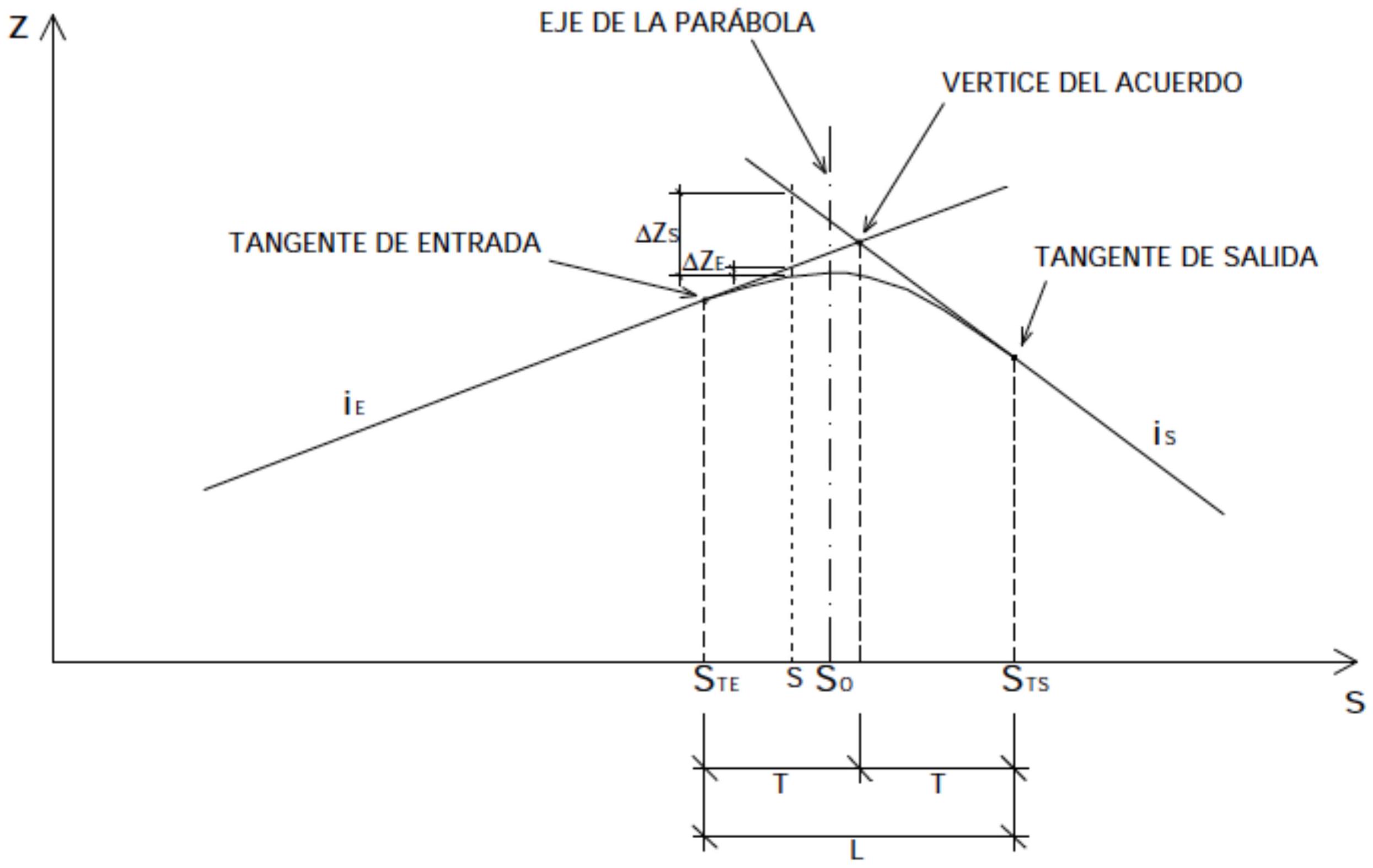
Geometric distribution of tangency points of entry and exit with respect to curve vertex is completely symmetric, fulfilling: \(T = L/2\).
V.1 MAXIMUM GRADIENT INCLINATION
Selection of maximum slope to implement in gradient requires systematic consideration of various technical and operational factors:
- Wheel-rail adhesion limitations: Friction coefficient available at wheel-rail interface establishes practical limit in magnitude of slope of order of 70‰.
- Technical capabilities of railway rolling stock:
- For passenger transport compositions: Under exceptional circumstances ramps up to 50‰ can be tolerated.
- For freight transport compositions: Inclination should not exceed 20‰.
- Nature and composition of traffic operating line (specialized traffic versus heterogeneous traffic).
- Starting capacity on ramp, manifesting in very short distances (typical length of compositions).
- Emergency braking capacity, intervening in greater distances, typically in range of 4 to 6 km for high speed operations.
Special considerations for vehicle stabling tracks:
Ideal longitudinal configuration in station infrastructures is horizontal, as this geometry eliminates operational complications associated with control of stopped compositions.
If impossible to implement perfectly horizontal gradient, uniform gradient with slopes limited between 1.5 and 3‰ must be chosen. In case necessary to implement vertical curves, parameter Kv must be greater than 5,000 m.
In accordance with Technical Specification for Interoperability relating to infrastructures of trans-European high-speed rail system, siding tracks dedicated to stabling compositions must not have slopes exceeding 2.5 mm/m.
These stabling tracks must be dimensioned to accommodate railway compositions up to 400 meters in length.
Limitations by extended length ramps:
It is technically undesirable to incorporate extensive sections characterized by continuous high slopes, as these configurations generate:
- Significant reduction of circulation speeds of compositions during ascent.
- Increase of braking distances during descent, negatively impacting operational safety.
- Increase of operating costs derived from greater energy consumption and expansion of travel times.
- Increase of maintenance and conservation costs of road infrastructure.
MAXIMUM GRADIENT INCLINATION
- Regulations: a) ADIF Regulations. Maximum ramp values established by this standard are:
| MAXIMUM RAMPS (\%) - N.R.V. 0-2-0.0. | |||||
|---|---|---|---|---|---|
| PROJECT SPEED ( \(\mathrm{Km} / \mathrm{h}\) ) | \(\mathrm{V}=140\) | \(140<\mathrm{v}=160\) | \(160<\mathrm{v}=200\) | \(200<\mathrm{v}=250\) | |
| NEW LINES AND DUPLICATION OF CURRENT LINES WITH ALIGNMENT MODIFICATION | NORMAL | 20 | 15 | 12.5 | 12.5 |
| EXCEPTIONAL | - | 20 | 15 | - |
- PURE PASSENGER TRAFFIC FOR \(\mathrm{V}>250 \mathrm{~km} / \mathrm{h}\) : MAXIMUM RAMP OF \(35 \%\).
- STATIONS: MAXIMUM RAMP OF \(2,5 \%\).
Regulations:
b) Technical Specification for Interoperability relating to infrastructure subsystem of trans-European high-speed rail system:
Maximum value of ramps and slopes may reach \(35 \%\), provided following conditions are respected:
- Average gradient slope over length of 10 km must be less than or equal to \(25 \%\).
- Maximum length on continuous ramp or slope of \(35 \%\) must not exceed 6,000 m . c) IOS-98:
Maximum admissible ramps in tunnels are:
- Mixed traffic lines: \(12,5 \%\).
- Exclusive passenger traffic lines: \(30 \%\).
V.2 ADMISSIBLE ACCELERATION IN VERTICAL CURVES
When a vehicle travels at speed ‘v’ a vertical curve of radius Rv, it is subjected to centrifugal acceleration:
\[a_{v}=\frac{v^{2}}{R_{v}}\]To respect passenger comfort this acceleration is limited to values ranging between 1 and 4% of ‘g’ (gravity value).
When a railway composition transits at speed v through a vertical curve of radius Rv, it is subjected to a vertical centrifugal acceleration characterized by:
\[a_{v}=\frac{v^{2}}{R_{v}}\]To ensure compliance with passenger comfort criteria, this vertical acceleration must be limited to values typically oscillating between 1 and 4% of gravitational acceleration (g).
Value of radius Rv has significant implications on configuration of earthworks and construction costs. French administration SNCF conducted specific research for TGV South-East project, proceeding to simulation tests using aircraft in flight.
These experimental tests were performed by Brétigny Flight Test Center, using an aircraft that in scheduled flight described controlled vertical sinusoidal trajectories. A group of passengers noted their subjective perceptions as function of acceleration magnitude and temporal spacing. Most sensitive passengers reported not perceiving accelerations of 0.045 g, while accelerations of 0.06 g were clearly perceived, especially in concave configuration curves.
Based on these experimental tests, SNCF established following normative limits for high speed operations:
| Normal value | Exceptional value | |
|---|---|---|
| Concave curve | \(a_v = 0,045 \, g\) | \(a_v = 0,06 \, g\) |
| Convex curve | \(a_v = 0,045 \, g\) | \(a_v = 0,05 \, g\) |
These acceleration limits translate into following minimum vertical curve radii:
| Normal value | Exceptional value | ||
|---|---|---|---|
| \(V = 300 \, \text{km/h}\) | Concave curve | \(R_V = 16.000 \, \text{m}\) | \(R_V = 12.000 \, \text{m}\) |
| Convex curve | \(R_V = 16.000 \, \text{m}\) | \(R_V = 14.000 \, \text{m}\) | |
| \(V = 350 \, \text{km/h}\) | Concave curve | \(R_V = 19.000 \, \text{m}\) | \(R_V = 18.500 \, \text{m}\) |
| Convex curve | \(R_V = 19.000 \, \text{m}\) | \(R_V = 21.000 \, \text{m}\) |
Acceleration limit of \(0,22 \, \text{m/s}^2\) established in European standard ENV 13803-1 seems to represent excessively restrictive value from perspective of operational practice.
A value of \(0,3 \, \text{m/s}^2\) constitutes reasonable minimum, considering that French TGV North of Europe line, projected for 350 km/h, implements as normal value a curve radius of 25,000 m, corresponding to acceleration of \(0,38 \, \text{m/s}^2\).
- ADIF Regulations. Maximum admissible acceleration in vertical curves fixed by standard is:
| MAXIMUM ADMISSIBLE ACCELERATION IN VERTICAL CURVES \(\mathrm{a}_{\mathrm{v}} \mathbf{( m} \mathbf{s}^{\mathbf{2}} \boldsymbol{)}\) - N.R.V. 0-2-0.0 | |||||
|---|---|---|---|---|---|
| PROJECT SPEED ( \(\mathrm{Km} / \mathrm{h}\) ) | \(\mathrm{V}=140\) | \(140<\mathrm{v}=160\) | \(160<\mathrm{v}=200\) | \(200<\mathrm{v}=250\) | |
| NEW LINES AND DUPLICATION OF CURRENT LINES WITH ALIGNMENT MODIFICATION | NORMAL | \(\leq 0,30\) | \(\leq 0,30\) | \(\leq 0,20\) | \(\leq 0,20\) |
| EXCEPTIONAL | 0,40 | 0,40 | 0,30 | 0,30 |
Comments: If vertical curve coincides with plan curve: \(\mathrm{a}_{\mathrm{v}} \leq 0,20\)
| PROJECT SPEED ( \(\mathrm{Km} / \mathrm{h}\) ) | \(\mathrm{V}=140\) | \(140<\mathrm{v}=160\) | \(160<\mathrm{v}=200\) | \(200<\mathrm{v}=250\) | |
|---|---|---|---|---|---|
| IMPROVEMENT OF CURRENT LINES BY WORKS (Track renovations and rehabilitations) | NORMAL | \(\leq 0,30\) | \(\leq 0,30\) | \(\leq 0,30\) | - |
| EXCEPTIONAL | 0,45 | 0,45 | 0,40 | - |
Comments: Maximum in convex curves: 0.40
If vertical curve coincides with plan curve: \(\mathrm{a}_{\mathrm{v}} \leq 0,20\)
| PROJECT SPEED (Km/h) | \(\mathrm{V}=140\) | \(140<\mathrm{v}=160\) | \(160<\mathrm{v}=180\) | \(180<\mathrm{v}=200\) | |
|---|---|---|---|---|---|
| ADAPTATION OF CURRENT LINES FOR TYPE A TRAIN CIRCULATION WITHOUT SPEED LIMITATION |
CONCAVE: | 0,50 | 0,50 | 0,45 | 0,45 |
| CONVEX: | 0,40 | 0,40 | 0,40 | 0,40 |
- Regulations:
- a) ADIF Regulations. As consequence, following minimum parameters result for vertical curves:
| MINIMUM VERTICAL CURVE RADIUS \(\mathbf{R}_{\mathbf{V}}(\mathbf{m})\) - N.R.V. 0-2-0.0. | |||||
|---|---|---|---|---|---|
| PROJECT SPEED ( \(\mathrm{Km} / \mathrm{h}\) ) | \(\mathrm{V}=140\) | \(140<\mathrm{v}=160\) | \(160<\mathrm{v}=200\) | \(200<\mathrm{v}=250\) | |
| NEW LINES AND DUPLICATION OF CURRENT LINES WITH ALIGNMENT MODIFICATION | NORMAL | 5,100 | 6,600 | 16,000 | 24,000 |
| EXCEPTIONAL | 3,800 | 4,900 | 10,000 | 16,000 | |
| IMPROVEMENT OF CURRENT LINES BY WORKS (Track renovations and rehabilitations) | NORMAL | 5,100 | 6,600 | 10,000 | - |
| EXCEPTIONAL | 3,400 | 4,400 | 7,700 | - |
MINIMUM PARAMETER IN CONVEX CURVES: 3,000 m MINIMUM PARAMETER IN CONCAVE CURVES: 2,000 m IF VERTICAL CURVE COINCIDES WITH PLAN CURVE MINIMUM PARAMETER WILL BE 5,000 m
| PROJECT SPEED \((\mathrm{Km} / \mathrm{h})\) | \(\mathrm{V}=140\) | \(140<\mathrm{v}=160\) | \(160<\mathrm{v}=180\) | \(180<\mathrm{v}=200\) |
|---|---|---|---|---|
| ADAPTATION OF CURRENT LINES FOR CIRCULATION OF TYPE A TRAINS WITHOUT SPEED LIMITATION |
3,100 | 4,000 | 5,000 | 6,900 |
- Regulations: b) European Standard ENV 13803-1
| MINIMUM VERTICAL CURVE RADIUS \(\mathrm{R}_{\mathrm{v}}(\mathrm{m})\) - ENV 13803-1 | ||
|---|---|---|
| Traffic Categories | Recommended maximum values ( \(\mathrm{V}_{\text {Max }}\) in km/h) | Permitted maximum values ( \(\mathrm{V}_{\text {Max }}\) in \(\mathrm{km} / \mathrm{h}\) ) |
| I: Mixed traffic lines, with passenger trains with maximum speeds between 80 and \(120 \mathrm{Km} / \mathrm{h}\). | \(0,35 \cdot \mathrm{~V}_{\text {Max }}{ }^{2}\) (2) | \(0,25 \cdot \mathrm{~V}_{\text {Max }}{ }^{2}\) (3) |
| IIa: Mixed traffic lines, with passenger trains with maximum speeds between 120 and \(160 \mathrm{Km} / \mathrm{h}\). | \(0,35 \cdot \mathrm{~V}_{\text {Max }}{ }^{2}\) | \(0,25 \cdot \mathrm{~V}_{\text {Max }}{ }^{2}\) (3) |
| IIb: Mixed traffic lines, with passenger trains with maximum speeds between 160 and \(200 \mathrm{Km} / \mathrm{h}\). | \(0,35 \cdot \mathrm{~V}_{\text {Max }}{ }^{2}\) | \(0,25 \cdot \mathrm{~V}_{\text {Max }}{ }^{2}\) (3) |
| III: Mixed traffic lines, with passenger trains with maximum speeds between 200 and \(300 \mathrm{Km} / \mathrm{h}\). | \(0,35 \cdot \mathrm{~V}_{\text {Max }}{ }^{2}\) | \(0,175 \cdot \bigvee_{\text {Max }}{ }^{2}\) (1) |
| IV: Mixed traffic lines, with passenger trains with speeds up to \(230 \mathrm{Km} / \mathrm{h}\) (or \(250 \mathrm{Km} / \mathrm{h}\) on the best lines) with vehicles incorporating special technical characteristics. | \(0,35 \cdot \mathrm{~V}_{\text {Max }}{ }^{2}\) | \(0,25 \cdot \bigvee_{\text {Max }^{2}}{ }^{2}\) (3) |
| V: Passenger traffic lines with maximum speeds between 250 and \(300 \mathrm{Km} / \mathrm{h}\). | \(0,35 \cdot \mathrm{~V}_{\text {Max }}{ }^{2}\) | \(0,175 \cdot \bigvee_{\text {Max }}{ }^{2}\) (1) |
(1) With tolerance of +10% in convex curve and +30% in concave curve.
(2) On lines where passengers may travel standing, \(R_v \leq 0.77 \cdot V_{Max}^2\) is recommended.
(3) Without going below radii of 2,000 m.
V.3 ABRUPT VARIATIONS OF VERTICAL ACCELERATION
Vertical curves are defined geometrically by parabolas with vertical axis, characteristics implying absence of transition curves between uniform gradient segments and vertical curve itself. This configuration generates discontinuous change in vertical acceleration at curve terminal points, originating oscillations in vehicle suspension systems and producing unpleasant sensations of discomfort in passengers.
When two vertical curves of opposite sign are coupled consecutively without inserting uniform gradient section, vertical acceleration jumps associated with each curve superimpose, producing significant adverse dynamic effects.
This configuration of consecutive curves generates following phenomena:
- Rapid unloading of suspension elements during transition from concave to convex configuration.
- Pronounced loading of suspension elements during transition from convex to concave configuration.
- Vertical acceleration jumps experienced by passengers, whose effective magnitude is gradually modified by suspension damping.
There are two design strategies to mitigate vertical acceleration jumps:
- Increase value of curve parameter (\(K_V\)), which increases radius of curvature.
- Design vertical curve incorporating geometric transition curves.
Both alternatives result in considerable increments of total length of vertical curve.
Solution currently adopted in railway engineering practice is first one, implementing following restrictions:
- Establish minimum lengths for vertical curves
- Establish minimum lengths for uniform inclination gradients
Justification of minimum vertical curve length:
It is imperative that sufficient time interval elapses between one vertical acceleration jump and next, allowing complete damping of vehicle suspension and avoiding superposition of dynamic effects that could cause significant structural oscillations.
Consequently, limitations are established on minimum permitted lengths for both uniform gradients and vertical curves.
Justification of minimum uniform gradient length:
It is feasible to design parabolic curve where vertical acceleration jump generated at Tangency point is individually admissible. However, when two vertical curves are placed immediately, acceleration jumps double, reaching considerably greater magnitudes.
For this reason, mandatory minimum length is established for uniform gradient segments located between two consecutive vertical curves, guaranteeing that vertical acceleration jumps do not superimpose. This configuration avoids negative effects on vehicle suspension systems and guarantees acceptable comfort conditions for passengers.
Illustrative case:
Let us consider high-speed line operating at \(v = 350 \, \text{km/h}\) with vertical curve parameter of \(K_V = 45.000 \, \text{m}\). In this configuration, vertical acceleration jump at tangency point turns out to be \(\Delta a_v = 0,21 \, \text{m/s}^2\), value considered admissible. However, if another vertical curve is immediately coupled without intermediate gradient, total resulting acceleration jump would be \(\Delta a_v = 0,42 \, \text{m/s}^2\) (equivalent to 4.2% of g), representing considerable and unacceptable acceleration value.
Limitations according to ADIF regulations:
ADIF technical regulations specify that minimum admissible length for uniform inclination gradient must be comprised between product of 0.4 times project speed and product of 0.5 times same speed.
| MINIMUM UNIFORM GRADIENT LENGTH (m) - N.R.V. 0-2-0.0. | ||||
|---|---|---|---|---|
| PROJECT SPEED ( \(\mathrm{Km} / \mathrm{h}\) ) | \(\mathrm{V}=140\) | \(140<\mathrm{v}=160\) | \(160<\mathrm{v}=200\) | \(200<\mathrm{v}=250\) |
| NEW LINES AND DUPLICATION OF CURRENT LINES WITH ALIGNMENT MODIFICATION | 70 | 80 | 100 | 100 |
| IMPROVEMENT OF CURRENT LINES BY WORKS (Track renovations and rehabilitations) | 70 | 80 | 100 | - |
Review Questions
What main function does cant perform in a railway curve?
Elevating outer rail with respect to inner one to reorient force resultant and eliminate lateral acceleration.
What name is given to configuration where resultant of centrifugal force and weight is perpendicular to track?
It is called theoretical cant or ideal cant (fully compensates centrifugal force).
How is cant deficiency (I) defined?
It is difference between theoretical cant (necessary to compensate centrifugal) and real cant implemented in track.
What comfort criterion limits uncompensated transverse acceleration for passenger according to text?
Maximum tolerable value without significant annoyance is situated around 1 m/s².
What parameter classifies train types (Normal, A, B, C, D) according to regulations?
They are classified according to maximum admissible values of uncompensated transverse acceleration they can withstand.
Bibliography
- Ferrocarriles. Apuntes de Clase. Jose Manuel Garcia Díaz de Villegas
- Infraestructuras Ferroviarias. Andrés López Pita
- Geometría y Calidad de la vía. Manuel Losada
- La geometría en el trazado de ferrocarriles