Railway Traction Systems and Adhesion Analysis

---

Table of Contents

1. Chapter I Longitudinal Dynamics
2. Chapter II Speed Profile Calculation
3. Chapter III Travel Time Calculation - Base run
4. Chapter IV. Electrification
5. Review Questions
6. Bibliography

---

Chapter I Longitudinal Dynamics

I.1. Introduction

Longitudinal dynamics constitutes a fundamental field in railway engineering that deals with the analysis and understanding of the interactions between the different forces acting on a train during its movement. These forces include the tractive effort generated by the motors, braking forces, gravitational effects caused by topography, and inertia forces associated with changes in speed. It is important to highlight that this analysis refers specifically to movement in the longitudinal direction of the train, clearly differentiating itself from vertical dynamics which considers movements perpendicular to the direction of travel.

The study of longitudinal dynamics allows identifying and developing three key areas of research and practical application in railway transport. Firstly, it is possible to calculate with precision the speed profiles and travel times in different line sections, considering technical and infrastructure limitations. Secondly, it allows determining the maximum loads that can be towed by a locomotive while maintaining established safety standards. Finally, it provides the necessary tools to estimate the energy consumption required in different operational scenarios.

I.2. General Approach

During the movement of a train along a railway line, different types of forces act simultaneously in different directions. We can classify them into two main categories according to their effect on the train’s movement. Firstly, there are forces that favor and contribute to the displacement of the train in the desired direction. The tractive effort provided by the traction motors constitutes the fundamental driving force that propels the train forward. When the train travels through downhill sections, the gravitational component also acts favorably to the movement, facilitating acceleration without requiring motor effort.

Conversely, there exists a set of forces that oppose and resist the movement of the train, limiting its speed and acceleration. The braking effort, which can be dynamic or continuous, is controlled by the driver to regulate speed and achieve safe stops. Resistance to motion, resulting from multiple factors such as friction in wheels and mechanical elements, aerodynamic resistance, and others, acts constantly against the movement. Additionally, when the train ascends ramps, the gravitational component acts as a resistive force opposing the advance.

The fundamental relationship describing train movement under these conditions is expressed by Newton’s second law adapted to the railway context. For the circulation of a vehicle or set of vehicles to be possible, the driving element must provide a tractive effort capable of overcoming the resistances opposing the movement. This fundamental relationship of motion is given by the expression:

\[E-R=\frac{P}{g} \cdot \gamma\]

Where \(P\) is the weight of the railway composition and \(\gamma\) is the acceleration that the effort E would produce in it.

I.3. Traction

Tractive effort constitutes the fundamental driving force originating the train’s movement, generated by the traction motor and subsequently transmitted to the driving wheels through the transmission system. At a deeper conceptual level, the motor torque acting on each axle is converted into a horizontal force applied at the wheel rim, which interacts with the rail generating a reaction of equal magnitude but opposite direction according to Newton’s third law. It is precisely this reaction of the rail on the wheel rim that provides the necessary traction to propel the locomotive and the entire composition forward.

The relationship between power, force, and speed constitutes a fundamental relationship in the analysis of mechanical systems, including locomotives. This relationship is expressed by the following equation:

\[\operatorname{Pot}(\text { watt })=F(\text { Newton }) \cdot v(m / s)\]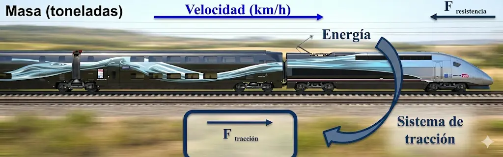

In railway transport practice, different units of measurement have been standardized throughout railway history. Regarding power, the kilowatt (kW) is commonly used, with the typical range for total locomotive power being between approximately 3100 kW and 5600 kW, although historically horsepower (CV/HP) is also used, where the equivalence is 1 CV = 750 W. For tractive effort or force, the most common units are decanewtons (daN) or kilograms-force (Kg), with the equivalence of 1 Kg = 1 daN (approximately 9.8 N). Speed is commonly expressed in kilometers per hour (km/h), with the equivalence to the international system being 1 km/h = (1/3.6) m/s.

To facilitate practical calculations in railway operations, direct relationships between these magnitudes in commonly used units have been developed:

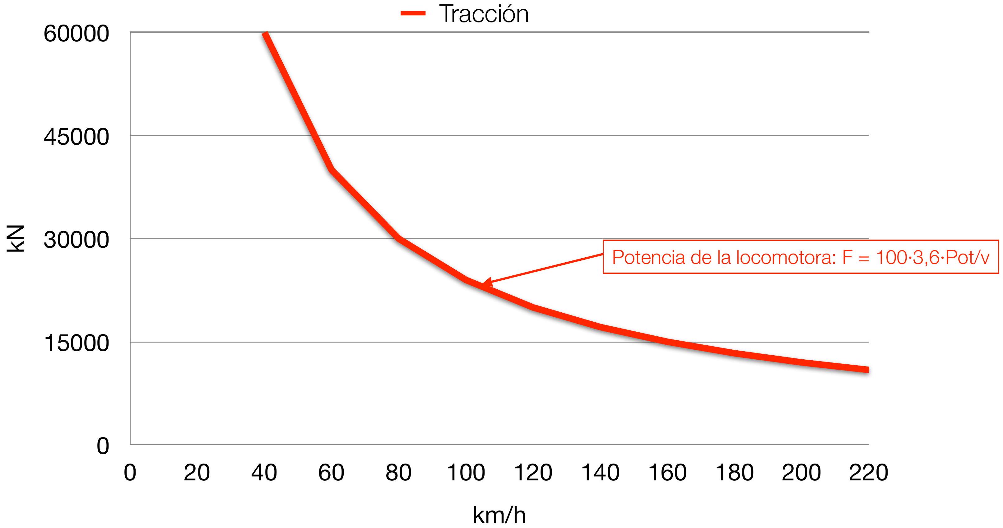
\[\begin{gathered} F(d a N)=100 \cdot 3,6 \cdot \operatorname{Pot}(k W) / v(k m / h) \\ F(K g)=270 \cdot \operatorname{Pot}(C V) / v(k m / h) \end{gathered}\]

• The effort-speed diagram constitutes a graphical tool of enormous utility that allows visualizing and analyzing the available traction capacity of a train as a function of its speed. From this diagram, it is possible to understand operational limitations and design optimal driving strategies.

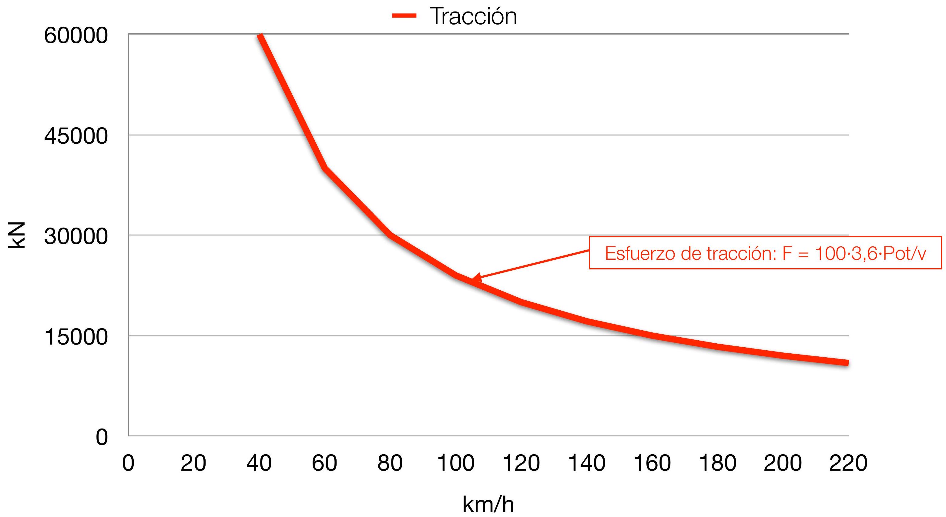
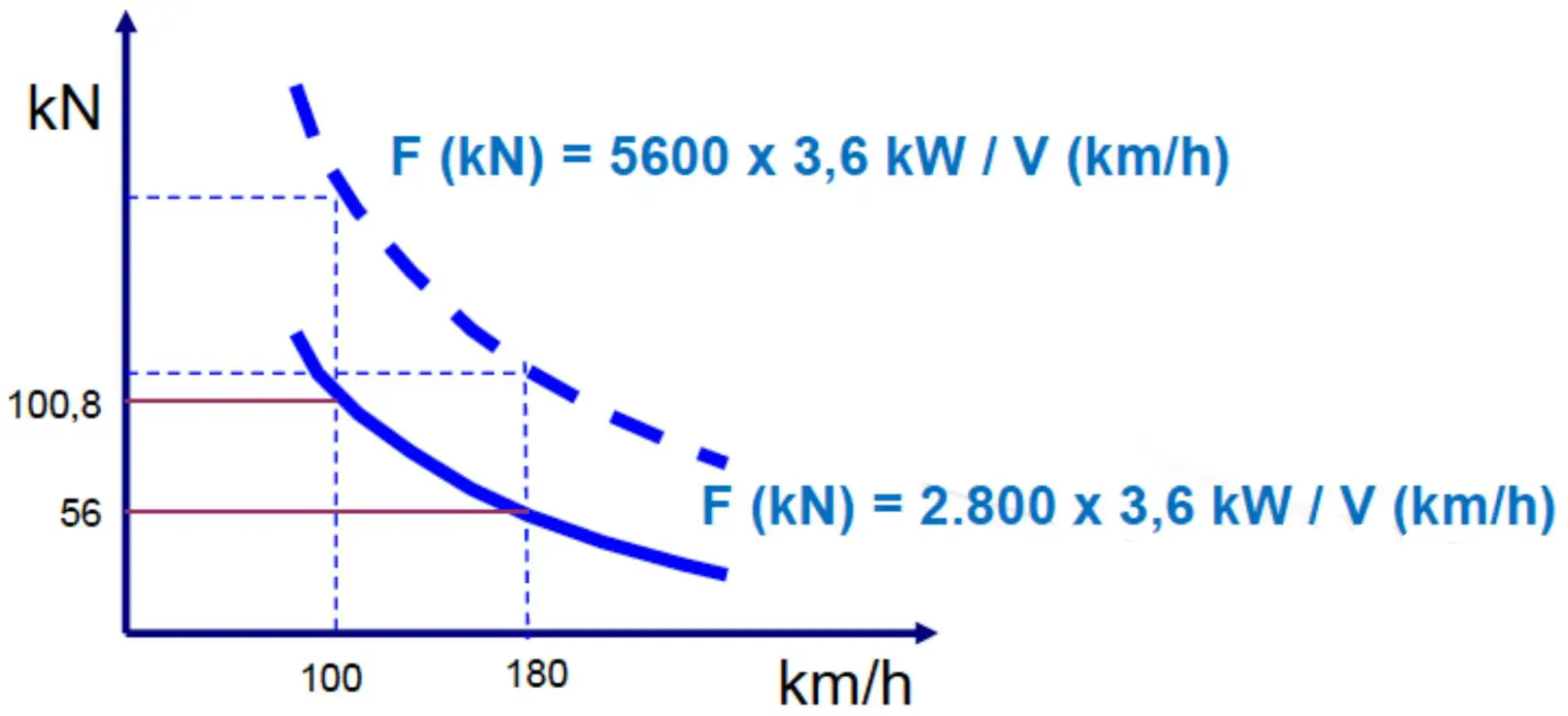
• The fundamental characteristics of this diagram show that available tractive effort presents variable behavior according to operational conditions. Tractive effort reaches its maximum values when the train is at low speeds, which is especially relevant during starting and initial acceleration phases. Conversely, with increasing speed, available effort decreases inversely proportionally, being limited mainly by the power available in the traction motor. Additionally, when the number of available motors in the composition is reduced, the total power and therefore the maximum efforts that can be achieved are also significantly reduced.

Consider as an example the machine 252 equipped with a single motor group of 2,800 kW:

I.4. Adhesion

Adhesion constitutes a fundamental concept in railway engineering describing the ability of train wheels to maintain contact with the rail without slipping. This property is critical for the safe and efficient operation of trains, especially during starting, accelerating, and braking maneuvers. It is important to highlight that the maximum tractive effort that can be transmitted from the locomotive to the rail cannot exceed that which would cause wheel slip on the rail.

The phenomenon of adhesion is based on the principle that there is an interaction between the wheel and the rail generating a friction force. This support without wheel slip on the rail constitutes adhesion, which presents an important characteristic: it will be greater the greater the weight pressing on the rail. Thus, adhesion is directly related to the mass of the locomotive’s driving axles.

For adhesion to be maintained, the following condition must be met:

\[F \leq \phi \cdot P_{a d h}\]

where \(\phi\) is the so-called coefficient of adhesion and \(P_{a d h}\) is the adhesive weight, i.e., the weight of the locomotive’s driving axles.

If during operation the condition \(F > \phi \cdot P_{a d h}\) occurs, adhesion is broken and the wheel begins to slide on the rail. In this situation, the friction coefficient decreases to a lower value \(\phi' < \phi\), increasing the acceleration of axle rotation and associated rotating masses. This phenomenon is known as wheel slip, and is an undesirable event in railway operation that reduces efficiency and can cause damage.

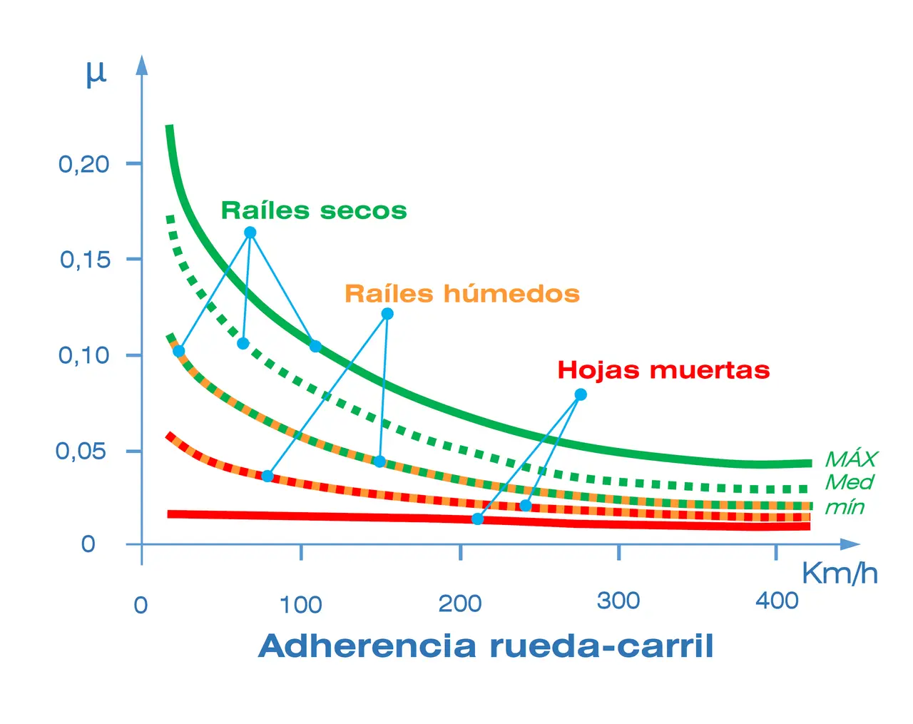
The variation of the coefficient of adhesion with speed is an aspect that has been widely studied in railway literature. The norm usually used by RENFE, based on extensive research, has the expression:

\[\phi_{v}=\phi_{0} \cdot\left[0.2155+\frac{33}{v+42}\right]\]

An alternative expression, simpler and widely used in modern practice, is the following:

\[\phi_{v}=\phi_{0} \cdot \frac{1}{1+0.01 \cdot v}\]

where \(\phi_{0}\) is the adhesion with the train stopped (initial condition) and \(v\) the speed in \(\mathrm{km} / \mathrm{h}\).

The maximum tractive effort a locomotive can exert is limited by available adhesion. This limitation is calculated as the product of the adhesive weight by the coefficient of adhesion:

\[E_{a d h}=P_{a d h} \cdot \phi_{v}\]

I.5. Traction and Adhesion

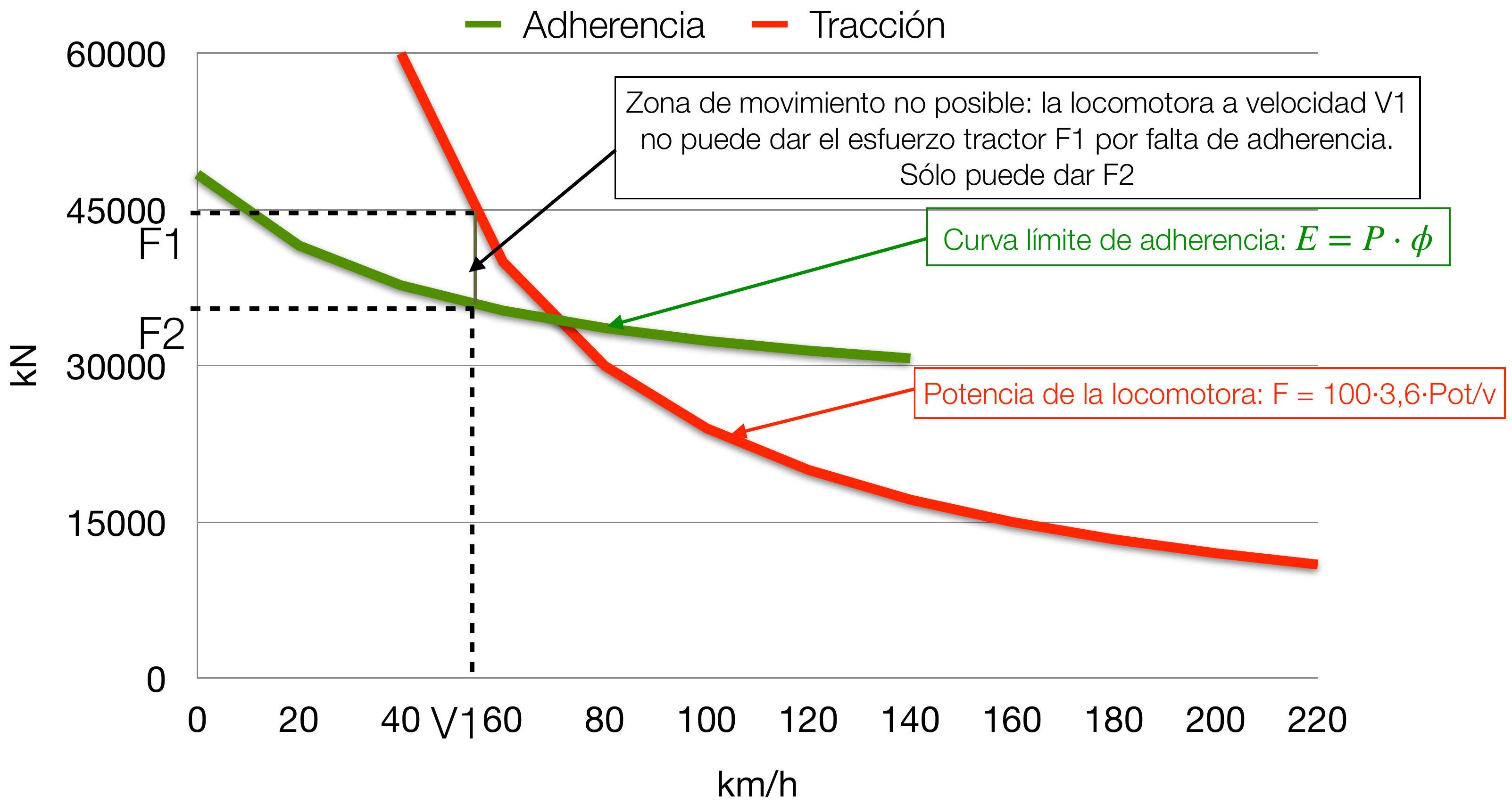
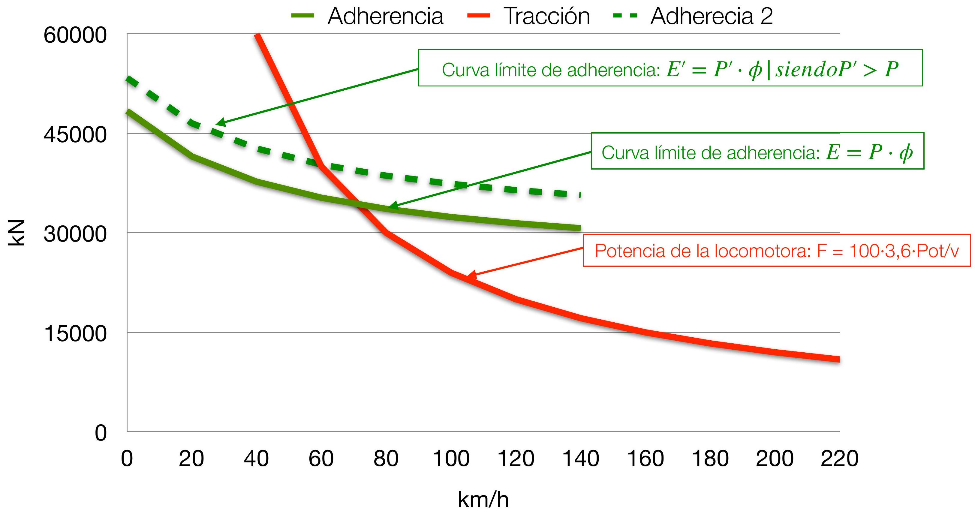
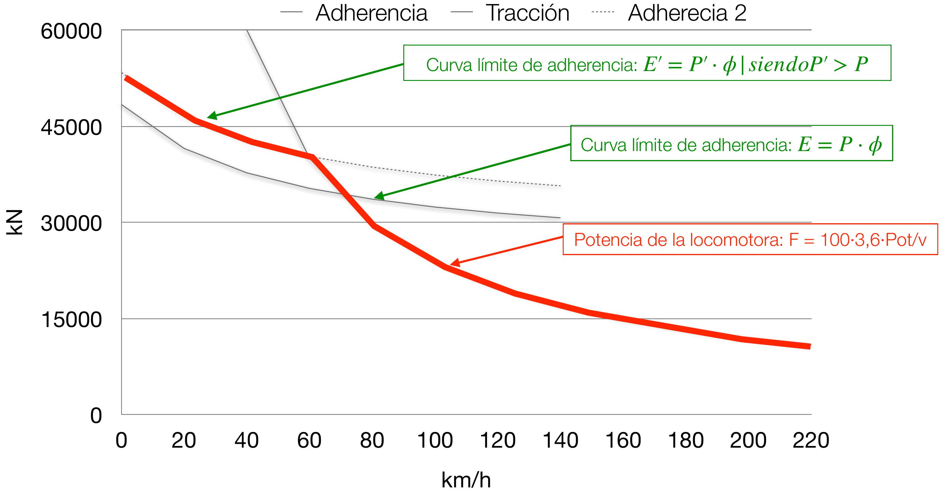
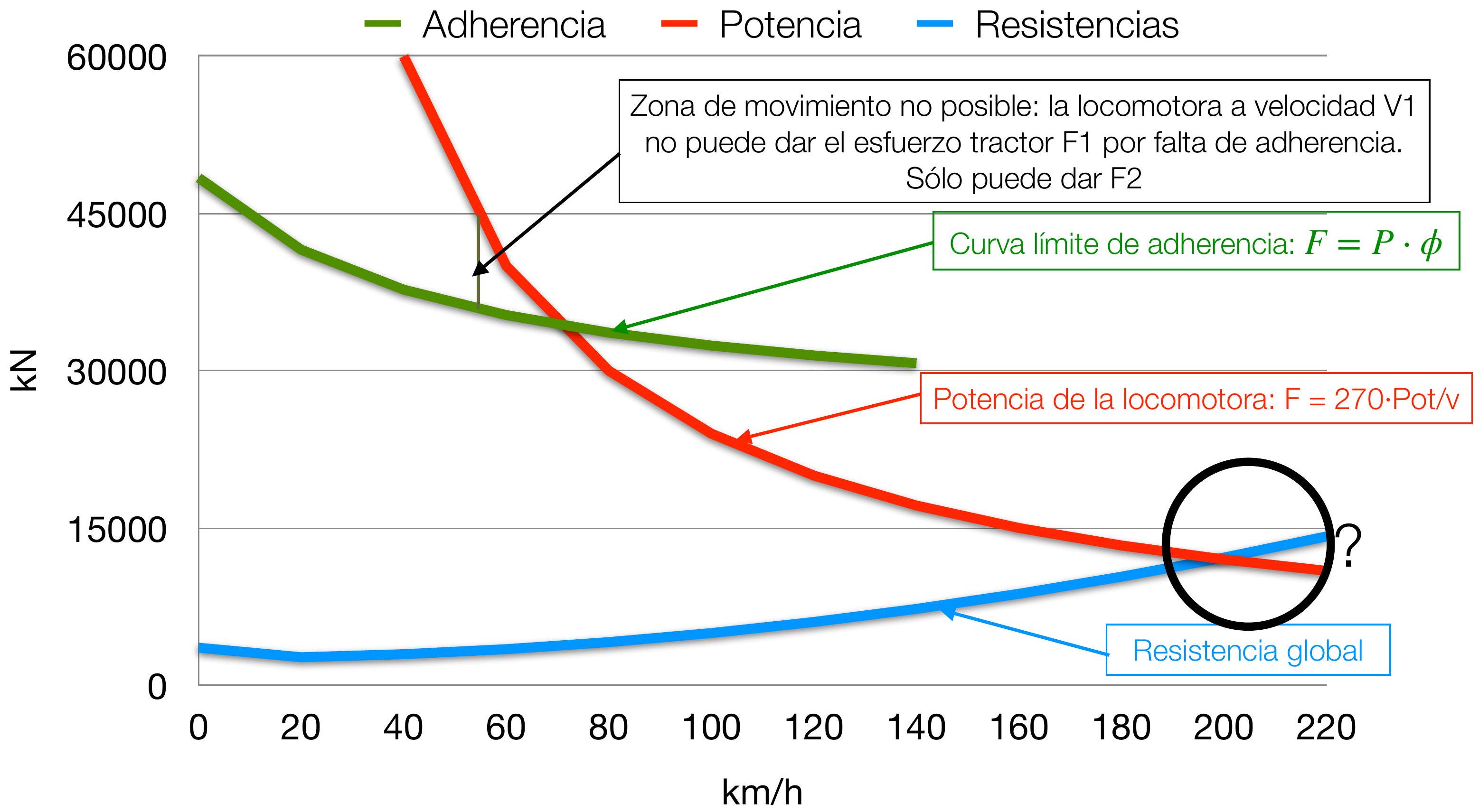
In analyzing the dynamic behavior of a locomotive, it is fundamental to consider simultaneously both limitations imposed by available power and limitations imposed by adhesion between wheels and rail. These two factors behave differently with speed and therefore generate different operational restrictions in different speed ranges.

When representing graphically the effort-speed relationship of a locomotive, considering only power limitation, the resulting curve is not asymptotic to the abscissa axis near the origin. This observation indicates that tractive effort cannot reach infinite values at low speeds, as might theoretically appear from the power equation. The physical reason for this limitation is that available adhesion between wheels and rail provides a maximum ceiling to the effort that can be transmitted.

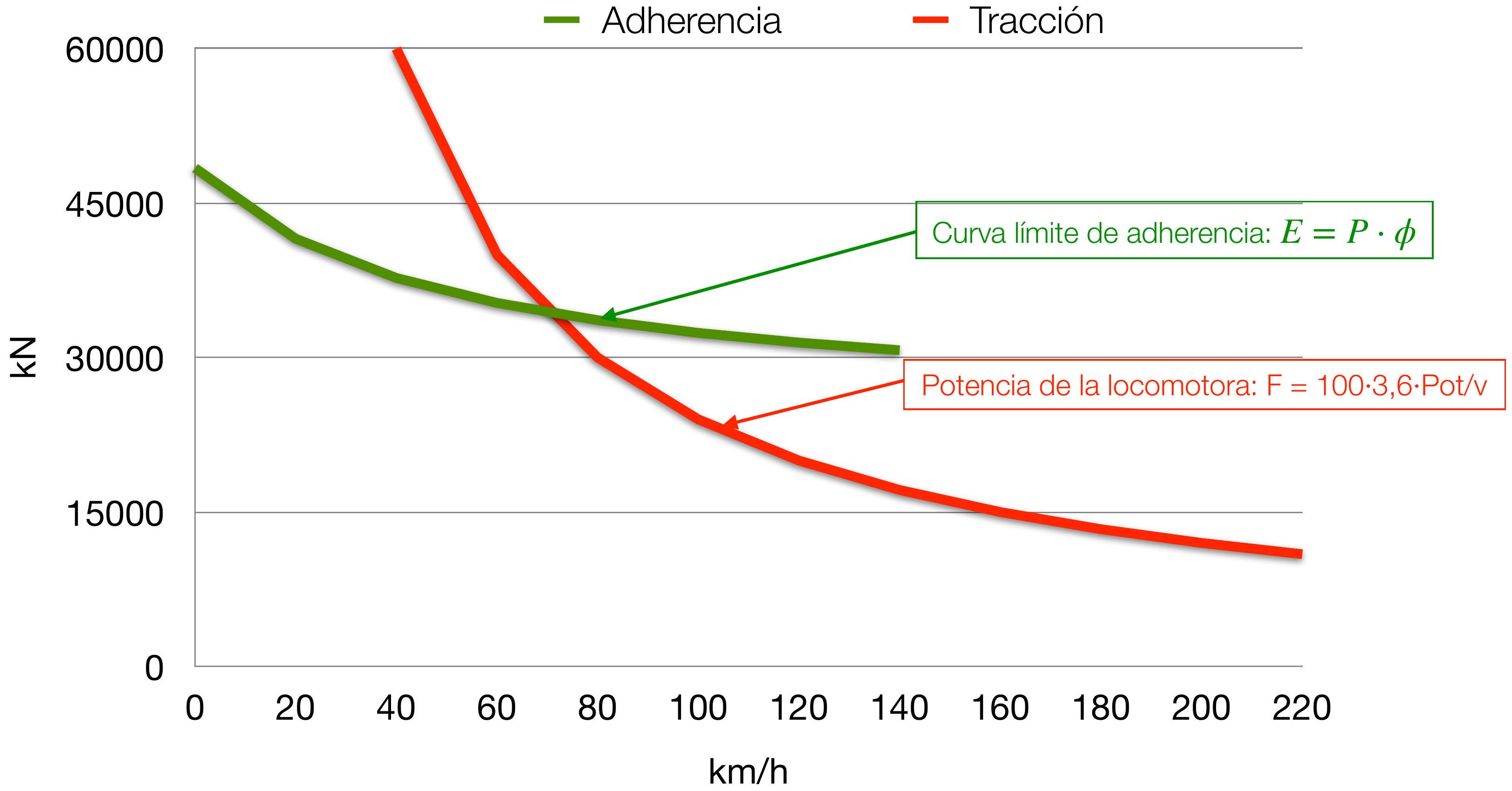
In train operational practice, it is common to find operating zones where performance is limited not by available power but by available adhesion. Similarly, there are operating zones where limitation is mainly due to traction motor power. Graphical representation of these two limitations on the same effort-speed diagram provides operational clarity.

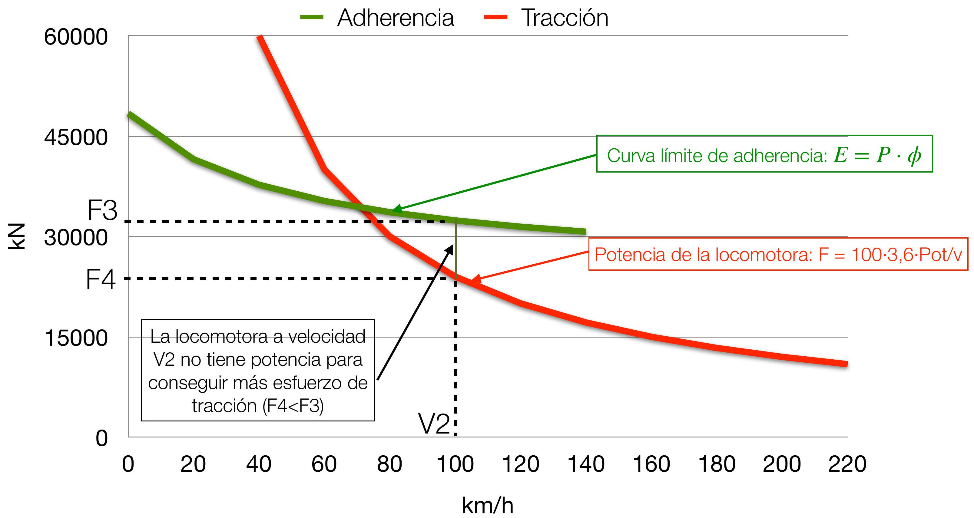
Available power constitutes a compromise between two fundamental physical magnitudes: drag force and movement speed. However, to achieve significant tractive force during critical maneuvers, sufficient adhesion is necessary, which can only be achieved by increasing the mass of the locomotive’s driving axles. This relationship between power, force, and mass illustrates fundamental compromises in locomotive design.

Interaction between traction and adhesion

The coefficient of adhesion (\(\phi\)) constitutes one of the most relevant and critical factors in freight transport operation, where high tractive forces are generally required to tow significant loads. To illustrate the importance of this parameter, consider a comparative example: two locomotives with identical available power, but with different masses, will present significantly different towing capacities. Specifically, a locomotive with a mass of 120 tons possesses a towing capacity approximately 50% higher than another with a mass of 80 tons, despite both having the same nominal power.

\[E_{a d h}=P_{a d h} \cdot \phi_{v}\]

An important concept emerging from this analysis is that a machine with greater mass can exert superior tractive effort at low speeds compared to another machine having more power but less mass. This capacity is especially critical during starting phases and in steep gradient conditions.

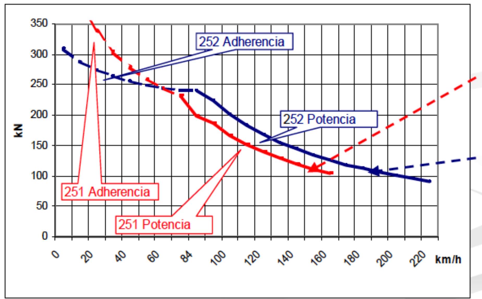
Two practical examples of locomotives in service illustrating this relationship are presented:

• Machine 251: Power 4,650 kW, mass 138 tons
• Machine 252: Power 5,600 kW, mass 92 tons

These examples demonstrate how, despite machine 252 having greater power, machine 251 with greater mass can achieve superior tractive efforts in certain speed ranges due to its greater adhesive weight.

I.6. Resistances to Motion

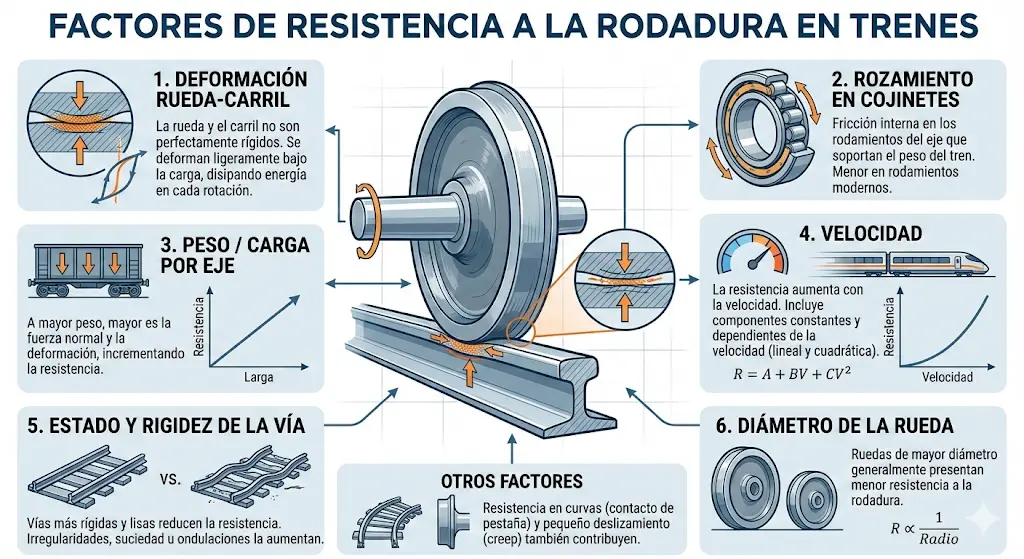
The movement of a train along a railway line is hindered by the presence of multiple resistive forces. Historically, the origins of these resistances have been identified as residing in specific characteristics of the rolling stock and line infrastructure, their magnitude being susceptible to influence by variable weather conditions. Regarding vehicle characteristics, resistances originate from multiple sources: friction existing in bearings and axle boxes, resistance to rotational movement of wheels on the rail, resistance due to rail deformation under train weight, and friction losses in various mechanical elements. Additionally, air resistance cannot be ignored, which presents an explicit dependence regarding relative speed between the train and outside wind.

Practical experience consistently shows that the sum of individual resistances calculated independently does not provide a result coinciding with total resistance to motion measured experimentally. For this reason, in engineering practice different resistances are combined using empirical expressions of parabolic nature, which present dependence on speed. For motor material cases, expressions appearing with linear and quadratic terms in speed are adopted:

\[r_{a}(d a N / t)=a+b \cdot v+c \cdot v^{2}\]

For towed vehicles, whether passenger coaches or freight wagons, specific resistance is generally evaluated from a general expression without a linear term in speed:

\[r_{a}(d a N / t)=a+c \cdot v^{2}\]

The components of resistance to motion can be classified into three main categories according to their physical origin:

• Mechanical Resistances (a): This category encompasses rolling resistance, including friction with the rail, rail deformation under load, and other rolling effects, as well as resistance due to internal system frictions, especially in axle boxes and other bearings.

• Resistances due to air intake (b): The movement of the train through the atmosphere requires displacing air found in its path, generating additional resistance.

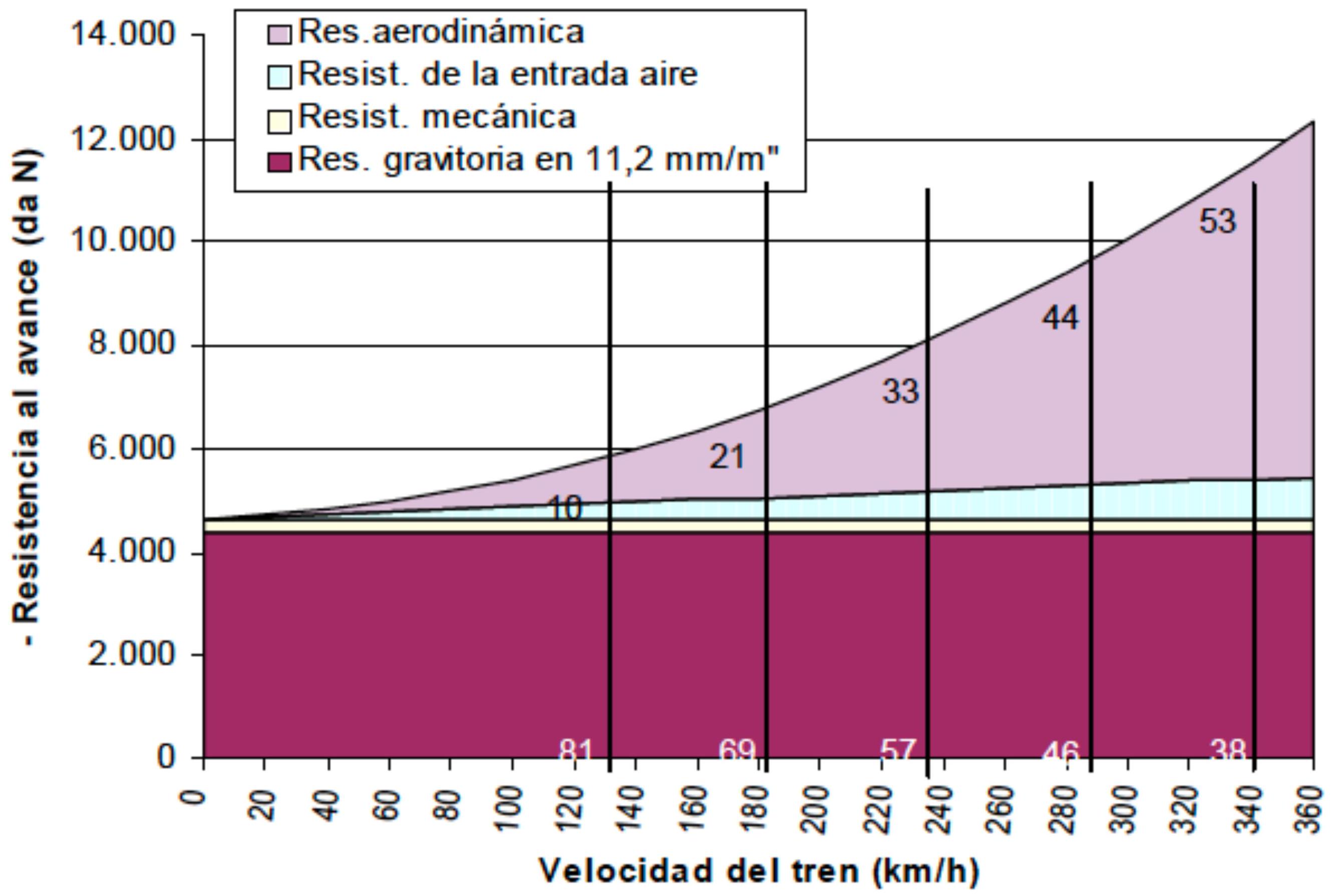
• Aerodynamic Resistances (c): These include pressure resistance resulting from frontal impact of the train and aerodynamic suction at the tail, as well as friction resistance generated by air flow over the train surface.

Total specific resistance to motion is then expressed as:

\[r_{a}(d a N / t)=a+b \cdot v+c \cdot v^{2}\]

TRAIN	Mass t	a	b	c
Locomotive BB	80	1.25	0.01	\(3.75 \cdot 10^{-4}\)
Locomotive CC	120	1.2	0.01	\(2.50 \cdot 10^{-4}\)
2 locomotives +6 coaches	400	1.15	0.00975	\(2.87 \cdot 10^{-4}\)
Classic passenger	Variable	1.5-2	0	\(2.22 \cdot 10^{-4}\)
Bogie freight	Variable	1.5-2	0	\(2.50 \cdot 10^{-4}\)
Classic freight	Variable	1.5-2	0	\(6.25 \cdot 10^{-4}\)
Alaris	177	1.5-2	0	\(6.25 \cdot 10^{-4}\)
TGV SudEst	418	0.562	0.00739	\(1.28 \cdot 10^{-4}\)
TGV Duplex	424	0.637	0.00755	\(1.26 \cdot 10^{-4}\)
ICE 3 Regional	231	0.735	0.00654	\(1.47 \cdot 10^{-4}\)

Resistance to motion

\[r_{a}(d a N / t)=a+b \cdot v+c \cdot v^{2}\]

TRAIN	Mass t	a	b	c
S100	421	0.603	\(8 \cdot 10^{-3}\)	\(1.120 \cdot 10^{-4}\)
S102	341	0.846	\(10 \cdot 10^{-3}\)	\(1.149 \cdot 10^{-4}\)
S103	485	0.736	\(7 \cdot 10^{-3}\)	\(1.112 \cdot 10^{-4}\)
S104	245	1.337	\(10 \cdot 10^{-3}\)	\(1.204 \cdot 10^{-4}\)
S120	275	0.819	\(3 \cdot 10^{-3}\)	\(1.164 \cdot 10^{-4}\)
S130	343	0.831	\(7 \cdot 10^{-3}\)	\(1.161 \cdot 10^{-4}\)
S730 (electric)	354	0.903	\(6 \cdot 10^{-3}\)	\(1.553 \cdot 10^{-4}\)
S730 (diesel)	354	0.903	\(1.4 \cdot 10^{-2}\)	\(1.508 \cdot 10^{-4}\)

Resistances due to railway infrastructure characteristics

The influence of the track on generating resistances to motion is fundamentally concretized in the characteristics of the line’s geometric layout, with the presence of curved sections and ramps or gradients being especially significant. These infrastructure elements generate additional resistances that must be considered in longitudinal dynamics calculations centered on:

Resistance due to curves:

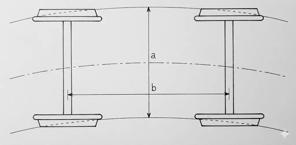
Resistance originating from train passage through curved sections of the line is generated as a result of three main mechanisms: solidarity of wheels and axles forcing vehicles to follow track curvature; parallelism of axles of different vehicles generating additional friction forces against the rail; and centrifugal force derived from circular motion kinematics. The general expression describing this resistance is:

\[F_{c}(d a N / t)=a \cdot f \cdot \frac{P}{R}+\frac{P \cdot f}{2 \cdot R} \cdot \sqrt{a^{2}+b^{2}}+\frac{P \cdot f}{R \cdot g} \cdot\left(V^{2}-V_{0}^{2}\right)\]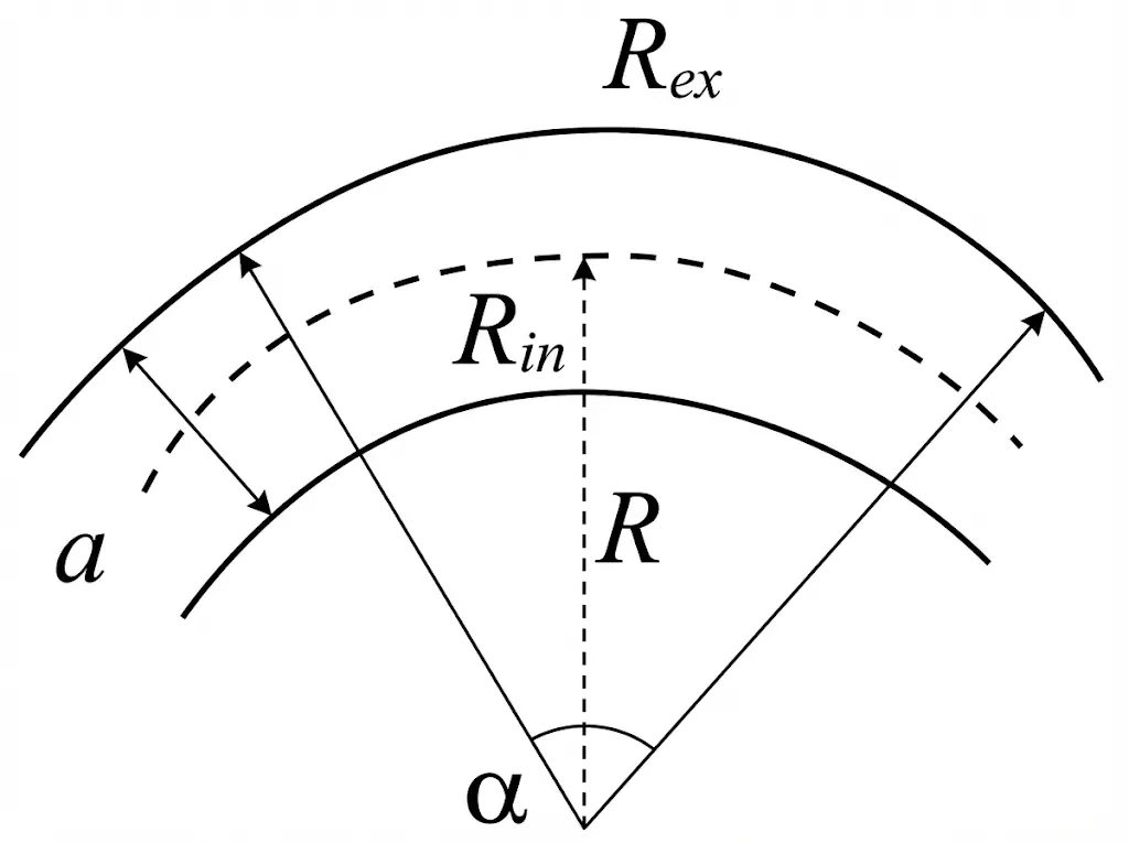

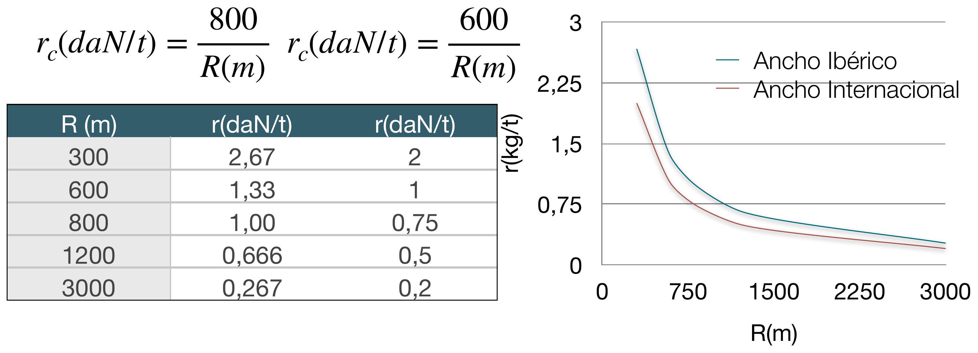
In Spanish operational practice, the infrastructure administration (Adif) employs specific simplified expressions for calculating resistances in curves, differentiating by track gauge:

\[r_{c}(d a N / t)=\frac{600}{R(m)} \quad \text{(standard gauge)} \quad r_{c}(d a N / t)=\frac{800}{R(m)} \quad \text{(Iberian gauge)}\]

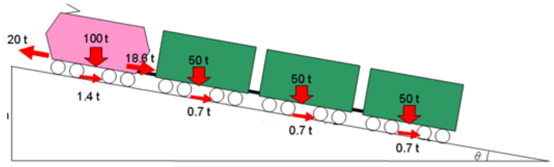
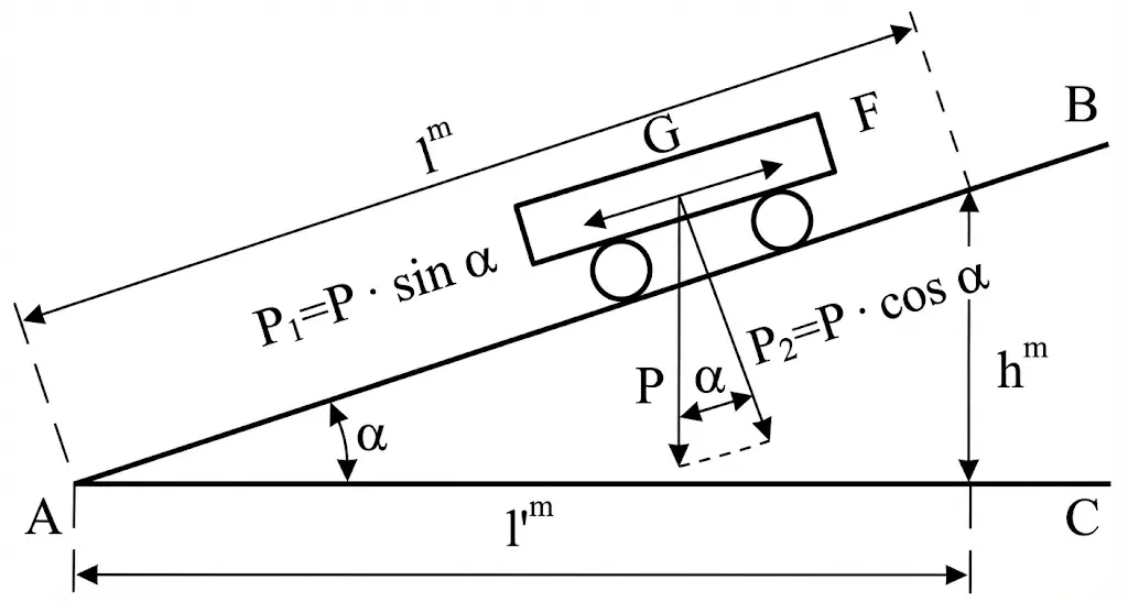
Resistance due to ramps:

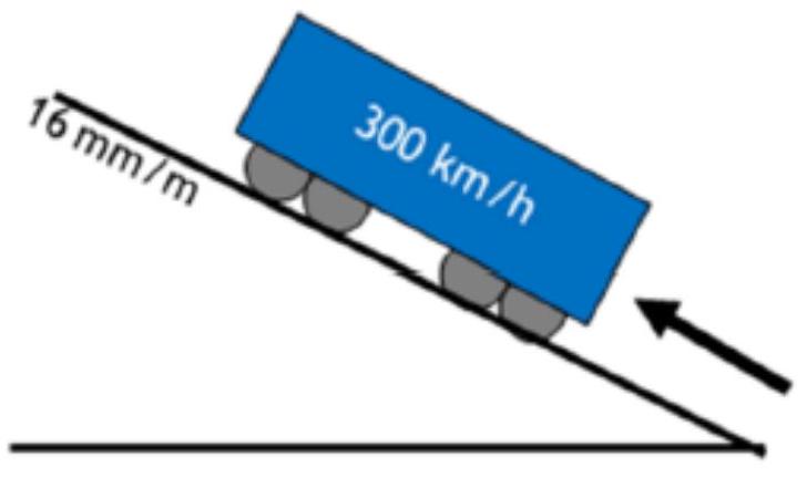
When a train must travel on an upward sloping section (ramp), additional work must be done to increase the train’s potential energy. Considering the usual scheme representing a ramp of gradient \(i=\operatorname{tg}(\alpha)\), it is possible to analytically deduce the supplementary effort such ramp generates during vehicle circulation. The deduction of this resistance is immediate from force equilibrium considerations:

\[r(d a N / t)=\frac{P \cdot i}{P}=i\]

On the other hand, in practical calculation applications, the concept of fictitious profile (L’) or equivalent fictitious ramp is used, which performs the joint consideration of resistance in curve and resistance in ramp. This magnitude is given by the expression:

\[L^{\prime}=\frac{800}{R(m)}+i\]

This simplified formulation allows performing unified analysis of geometric layout characteristics, facilitating computational calculation.

Resistances to motion

\(\mathrm{i}(\mathrm{mm} / \mathrm{m})\)	\(\mathrm{r}(\mathrm{daN} / \mathrm{t})\)
2	2
12	12
20	20
35	35

\[r(d a N / t)=\frac{P \cdot i}{P}=i\]

Total resistance at constant speed:

When a train travels at constant speed, the total specific resistance that must be overcome constitutes the sum of all partial resistances previously described:

\[r_{t}(k g / t)=r_{a}+r_{c}+r_{i} \rightarrow R_{t}(k g)=R_{a}+R_{c}+R_{i}\]

Inertia Resistance:

Inertia resistance constitutes a resistance opposing any change in train speed, regardless of its direction (acceleration or deceleration). This resistance presents a fundamental characteristic: its magnitude depends directly on the total mass of the train and the magnitude of acceleration (or deceleration) attempted. Mathematically, if \(a\) is defined as acceleration expressed in cm/s², specific inertia resistance is calculated by the following relationship:

\[\begin{aligned} R_{i n}=\frac{P}{g} \cdot \frac{d v}{d t}=\frac{P(\mathrm{~kg})}{g\left(\mathrm{~cm} / \mathrm{sg}^{2}\right)} \cdot a\left(\mathrm{~cm} / \mathrm{sg}^{2}\right)=P \cdot a(\mathrm{~kg}) \\ r_{i n}=\frac{R_{i n}}{P}=\frac{P \cdot a}{P}=a(\mathrm{~kg} / \mathrm{t}) \end{aligned}\]

When all these resistive effects are integrated into an effort-speed diagram representing train behavior under different operating conditions, a complete representation of available dynamic performance is obtained:

I.7. Traction Curve

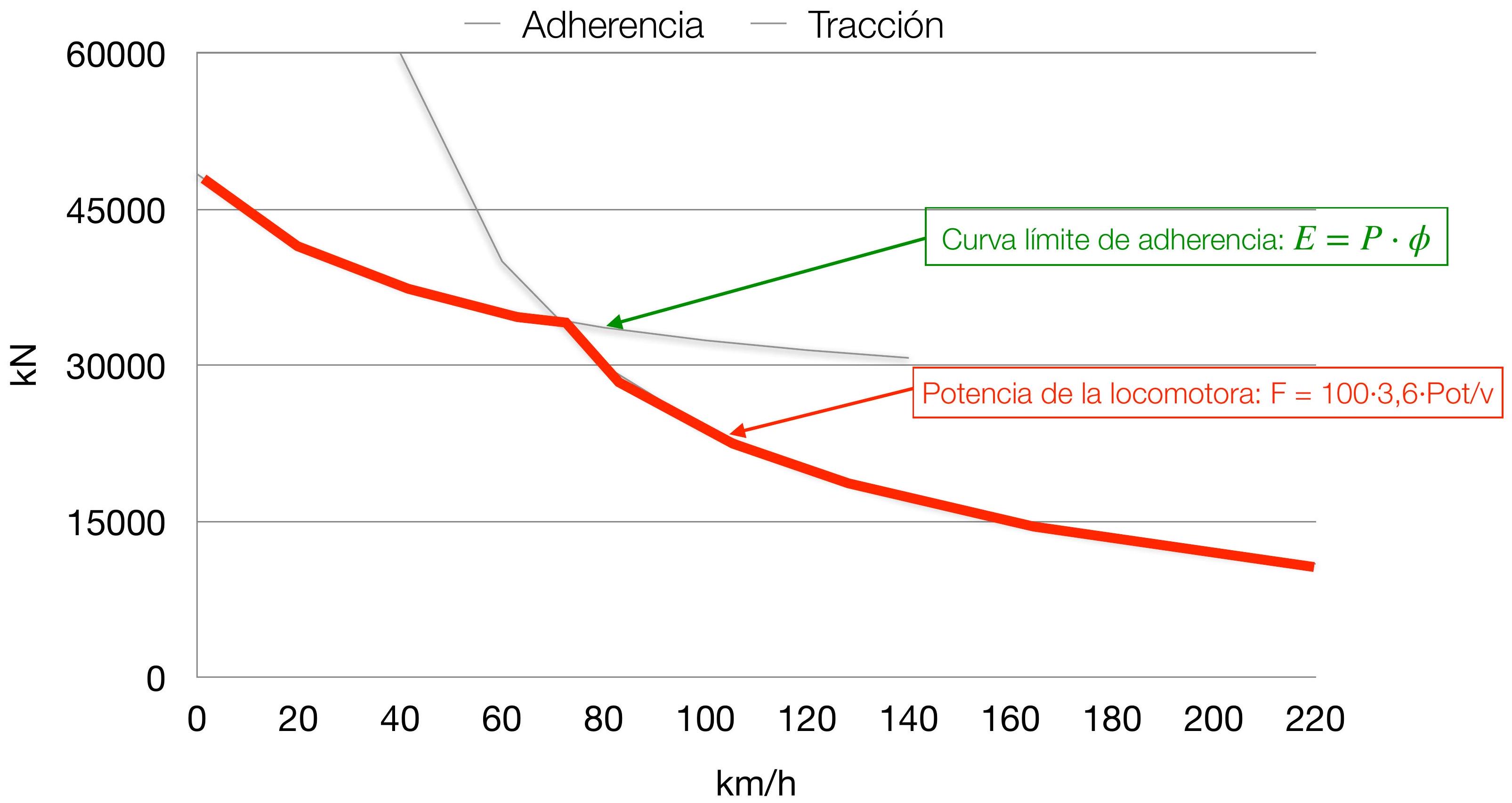
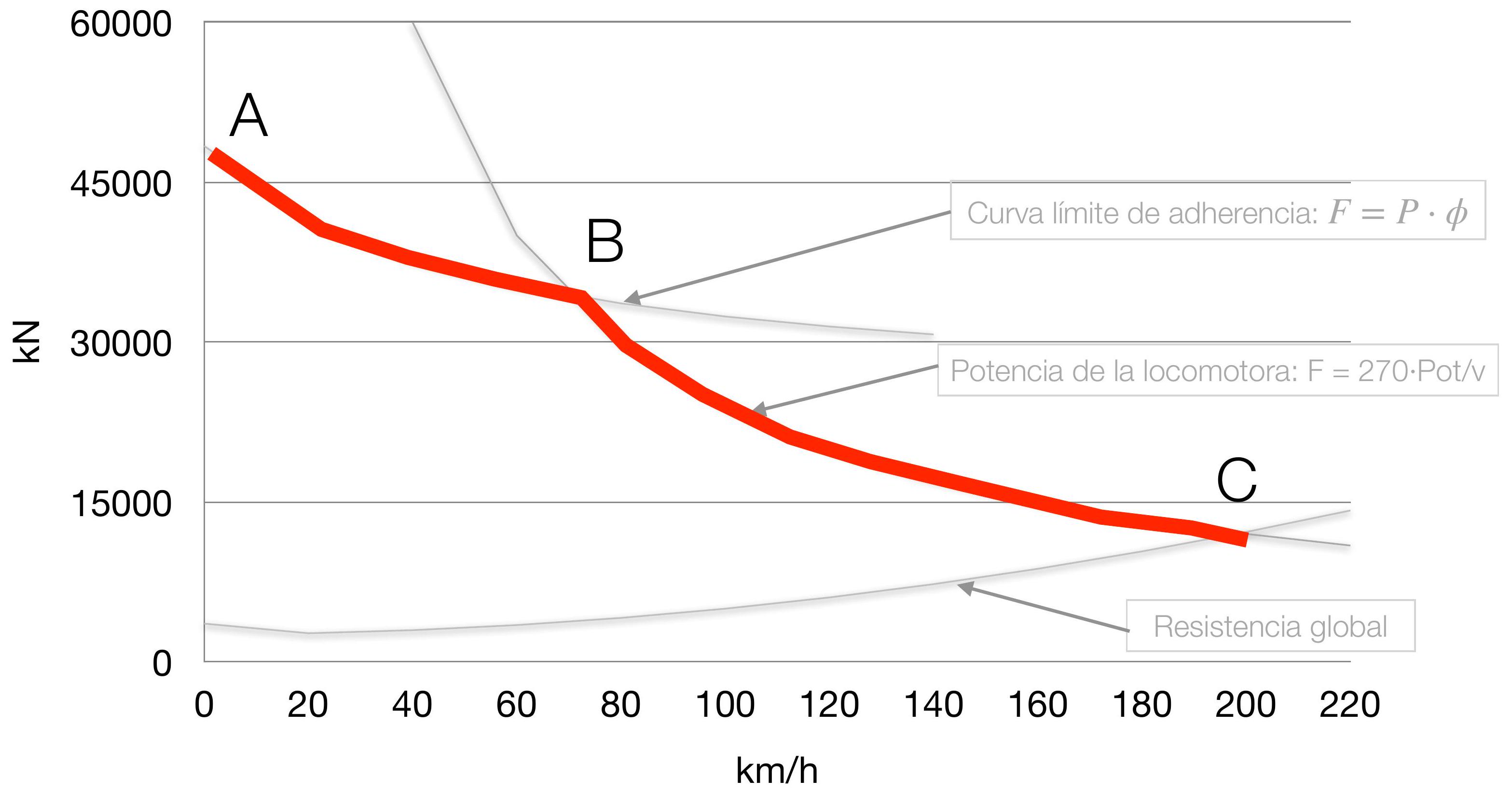
The process of train movement from rest conditions constitutes a complex dynamic process in which transitions occur between different operating regimes. Initially, movement begins at zero speed from point A, evolving along the available adhesion curve as the train progressively increases its speed, and reaching point B where transient limitation is adhesion. Subsequently, speed continues to increase following the power availability limitation curve, transitioning from point B to point C. At point C, the available effort curve (both by adhesion and power) intersects with the train’s global resistance curve which includes all resistive terms. At this intersection point, the train reaches its maximum possible speed for given operational conditions.

I.8. Dynamics on Ramps and Gradients

Train dynamic behavior on a mountainous layout presents significantly different characteristics to movement on horizontal track. The presence of gradients and ramps introduces modifications in force balance fundamentally affecting train operational performance.

Behavior on ramps (upward movement):

When a train travels upwards on a ramp, the gravitational component of weight acts directly opposite to movement, behaving as an additional resistive force added to the train’s natural resistance to motion. Consequently, to maintain constant speed on a ramp, the train requires significantly higher tractive effort than necessary on an equivalent horizontal section.

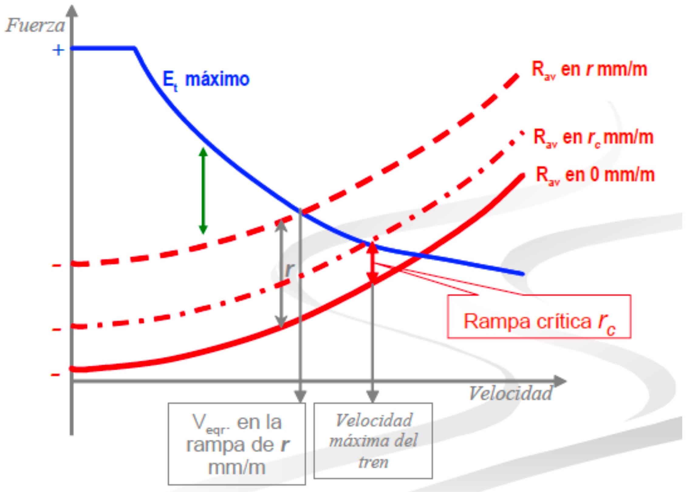
The equilibrium speed for a given ramp is defined as the maximum speed that can be achieved on that specific ramp, maintaining tractive effort equal to total resistance (including gravitational component). The concept of critical ramp is especially important: defined as the steepest gradient in which the train is capable of reaching its theoretical maximum speed. For ramps steeper than critical ramp, maximum achievable speed will be lower than train nominal maximum speed.

Behavior on gradients (downward movement):

In contrast to ramps, when a train travels downwards on a gradient, the weight’s gravitational component acts in the same direction as movement, effectively behaving as an additional driving force. This circumstance significantly reduces the tractive effort requirement necessary to maintain a determined speed.

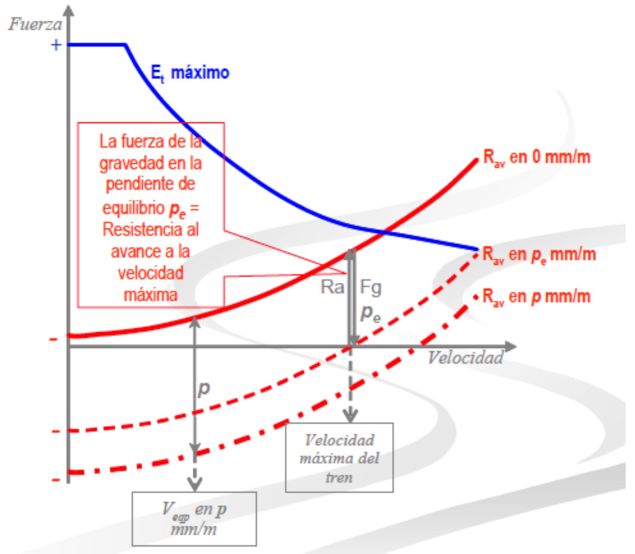
The concept of equilibrium gradient has particular operational importance: defined as that gradient in which the train in a condition of coasting without traction (drifting) precisely maintains its maximum speed. On gradients steeper than equilibrium gradient, the train tends to accelerate, requiring use of brakes to maintain maximum authorized speed. On gradients gentler than equilibrium gradient, the train requires additional traction to maintain maximum speed.

I.9. Resistances at Start

In practical train operation, the starting phase from rest presents characteristics significantly different from those of normal running movement. If only standard resistance to motion expressions evaluated at zero speed (v=0) were applied, resulting values would not represent observed experimental reality. Empirically, the resistance required to initiate train movement is notably greater than predicted by such theoretical models.

It has been determined by practical studies that to start a railway vehicle an effort of the order of 10 Kg/t is necessary, significantly higher than typical value of 1-1.5 Kg/t required when the train is already circulating in normal conditions. To this starting resistance must be added the effort required to impart initial acceleration to the train (termed inertia resistance), whose magnitude varies according to type of train considered:

Train Type	Minimum Starting Acceleration
Freight Trains	2 to 5 cm/s²
Conventional Passenger Trains	8 to 10 cm/s²
Railcars and Multiple Units	50 to 100 cm/s²
High Speed Trains (AVE)	80 to 100 cm/s²
Metro Systems	110 to 120 cm/s²

Railway infrastructure administration (Adif) adopts standard values for calculation of resistances at start. For a horizontal and straight line, standard specific resistance is 7 daN/t. This figure consists of two components: 4 daN/t correspond to minimum effort necessary to overcome static resistance and initiate movement, whilst remaining 3 daN/t represent accelerating effort required to achieve start in operationally acceptable time.

Starting phase on ramp constitutes most critical scenario from operational viewpoint, since it requires overcoming simultaneously starting resistance, inertia resistance and ramp gravitational component. To facilitate practical calculation and rolling stock dimensioning, normative values relating specific starting resistance with gradient magnitude have been established:

Specific Resistance at Start (daN/t)	Gradient (mm/m)
7	<15
8	15-20
9	21-25
10	26-29
11	30-33
12	34-37
13	38-41
14	42-45
15	>45

It is important to note that as ramp magnitude increases, required specific resistance increases proportionally. This phenomenon is because couplings and couplers between coaches or wagons experience greater structural stresses, generating additional resistances associated with elastic deformation of these elements.

Available adhesion at start constitutes a fundamental physical limitation that cannot be exceeded without producing wheel slip. This limitation is expressed by:

\[E_{\phi_{0}}(k g) \leq 1000 \cdot \phi_{0} \cdot P_{\text {locomotive }}(t)\]

Simultaneously, total effort to be overcome to surmount all resistances at start is determined by:

\[E(k g)=\left(P_{l o c}+P_{r e m o l}\right) \cdot\left(r_{a}+i\right)\]

To ensure start can be performed without producing wheel slip, it is imperative to verify:

\[\left(P_{l o c}+P_{r e m o l}\right) \cdot\left(r_{a}+i\right) \leq 1000 \cdot \phi_{0} \cdot P_{l o c}(t)\]

Through this condition it is possible to calculate maximum towable load by any locomotive in critical starting conditions.

TABLE 9.2 TOWABLE LOAD AT START FOR TWO REFERENCE SITUATIONS
Data	Passenger Train	Freight Train
Locomotive	BB (direct current)	BB (monophasic)
	of 80 t	of 84 t
Ramp	8%	10%
Curve Radius		400 m
Resistance
Specific at start
	2da N/t	\(1.5 \mathrm{da} \mathrm{N} / \mathrm{t}\)
Acceleration	\(8 \mathrm{~cm} / \mathrm{sec}^{2}\)	\(2 \mathrm{~cm} / \mathrm{sec}^{2}\)
Coefficient of
Calculations
Maximum effort at start	\(80 \mathrm{t} \times 0.2=16.000 \mathrm{daN}\)	\(84 \mathrm{t} \times 0.35=29.400 \mathrm{daN}\)
Specific effort at start t	2 (start) +
		\(\begin{gathered} 1.5 \text { (start) + } \\ 2 \text { (acceleration) + } \\ 10 \text { (ramp) + } 2 \text { (curve) } \\ =15.5 \text { da N/t } \end{gathered}\)
Total load at start (Q + L) (towed material	\((\mathrm{Q}+\mathrm{L})=\frac{16.000}{18} \approx 880 t\)	\((\mathrm{Q}+\mathrm{L})=\frac{29.400}{15.5}=1.896 \mathrm{t}\)
+ locomotive)
Load startable (Q) by locomotive
	\(\mathrm{Q}=880-80 \mathrm{t}=800 \mathrm{t}\)	\(Q=1.896-84=\sim 1.800 t\)

I.10. Hook Effort

In context of railway dynamics, hook effort is technically defined as net force available at locomotive coupling hook. This magnitude is calculated as total effort provided by traction motor, minus amount of effort locomotive needs to overcome resistances acting on its own structure considered as additional vehicle in composition.

Railway vehicles are provided with hooks or couplers designed for their mechanical interconnection. These coupling systems present structural resistance limitations determined by engineering criteria. Characteristic resistance of these couplers typically oscillates between 70 and 85 tons. To avoid exceeding material elastic limit and ensure adequate useful life, safety coefficients of 2.4 are adopted in design. Consequently, admissible tensile efforts that can be applied in sustained manner are:

• For nominal couplers of 70 tons: admissible effort of 30 tons
• For nominal couplers of 85 tons: admissible effort of 36 tons

To ensure couplings do not break during operation, following condition must be met at moment of start:

\[30 \mid 36 \cdot 10^{3} \geq P_{\text {remol }} \cdot\left(r_{a}+i\right)\]

I.11. Towable Load

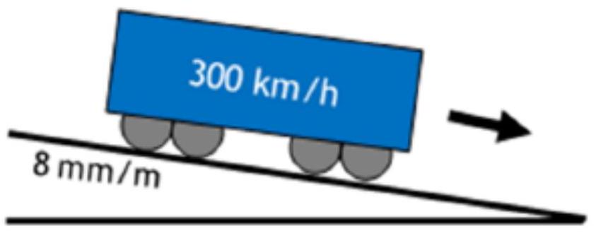
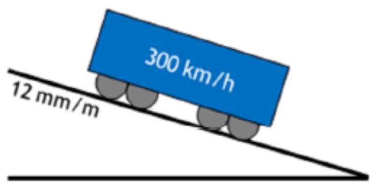
Dimensioning of railway compositions requires knowing maximum towing capacity of available locomotives. This capacity is function of multiple variables, including type of towed vehicles, unit mass, their length and maximum permitted speed. In context of freight transport, these parameters acquire critical importance, especially when considering starting conditions on steep ramps. Technical characteristics of different wagon types are presented below, followed by specific towing capacities for different locomotives under distinct operating conditions (gradient of 12‰ and 18‰):

FREIGHT (12 %o)

LOCOM.	v. max.	WEIGHT	LEN.	MAX. TOWED LOAD	OPEN	CLOSED	PLATFORMS			HOPPERS	TANKERS
							NORMAL	CARS	CONTAINERS
601.E	120	130	22.41	2125	371	509	642	1318	470	421	398
601.D	120	130	22.41	2159	377	517	653	1340	478	427	405
335	120	123	23.02	1890	332	454	572	1171	420	376	356
269.85	100	176	17.27	2220	374	516	652	1345	476	425	403
252	220	90	20.40	1200	214	291	365	741	269	242	229
253	140	87	18.90	1530	271	371	467	956	343	307	291

FREIGHT \((18 %)\)

LOCOM.	v. MAX.	WEIGHT	LEN.	MAX. TOWED LOAD	OPEN	CLOSED	PLATFORMS			HOPPERS	TANKERS
							NORMAL	CARS	CONTAINERS
601.E	120	130	22.41	1517	264	361	453	923	334	299	283
601.D	120	130	22.41	1522	265	362	455	926	335	300	284
335	120	123	23.02	1340	235	320	401	814	296	266	252
269.85	100	176	17.27	1580	262	360	453	929	332	297	282
252	220	90	20.40	880	158	213	265	533	197	178	169
253	140	87	18.90	1080	192	261	327	664	242	217	206

Chapter II Speed Profile Calculation

The actual travel speed of a train along a railway line results from the combination of multiple interconnected factors. Among the most significant are acceleration and braking capability available in rolling stock, specific type of train considered, traction technology employed (diesel, electric AC or DC), geometric characteristics of layout (gradients, curves, curvature radius), meteorological conditions, and regulatory restrictions.

Under ideal operational conditions, the driver responsible for the train has certain margins of operative flexibility allowing modulation of train progress. These margins can be exploited strategically to optimize energy consumption, balancing speeds, accelerations and decelerations intelligently. However, it is necessary to consider that there are imperative speed limitations that must be respected under all operational circumstances. These limitations are established at special track switches, tunnels with reduced sections (to avoid adverse aerodynamic effects like piston effect), metal bridges with restrictions, and zones with obstacles close to railway infrastructure. A fundamental and indispensable tool in modern railway engineering is the speed diagram or speed profiles. These diagrams are habitually represented in speed-space coordinates, where abscissa axis represents distance traveled along railway line and ordinate axis represents train speed at each point. These diagrams acquire special utility when employed jointly with an additional diagram showing gradients and ramps of layout, allowing visualization of mutual influence between topography and speed profile.

From careful analysis of speed diagrams it is possible to study and predict multiple parameters of operational interest and comfort. Among these are efforts transmitted to railway infrastructure by train passage under different dynamic regimes, as well as comfort parameters for travelers related to accelerations and decelerations produced. Subsequent analysis describes in detail constituent elements of a representative speed diagram:

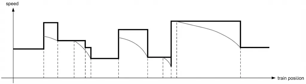
II.1. Speed Profiles

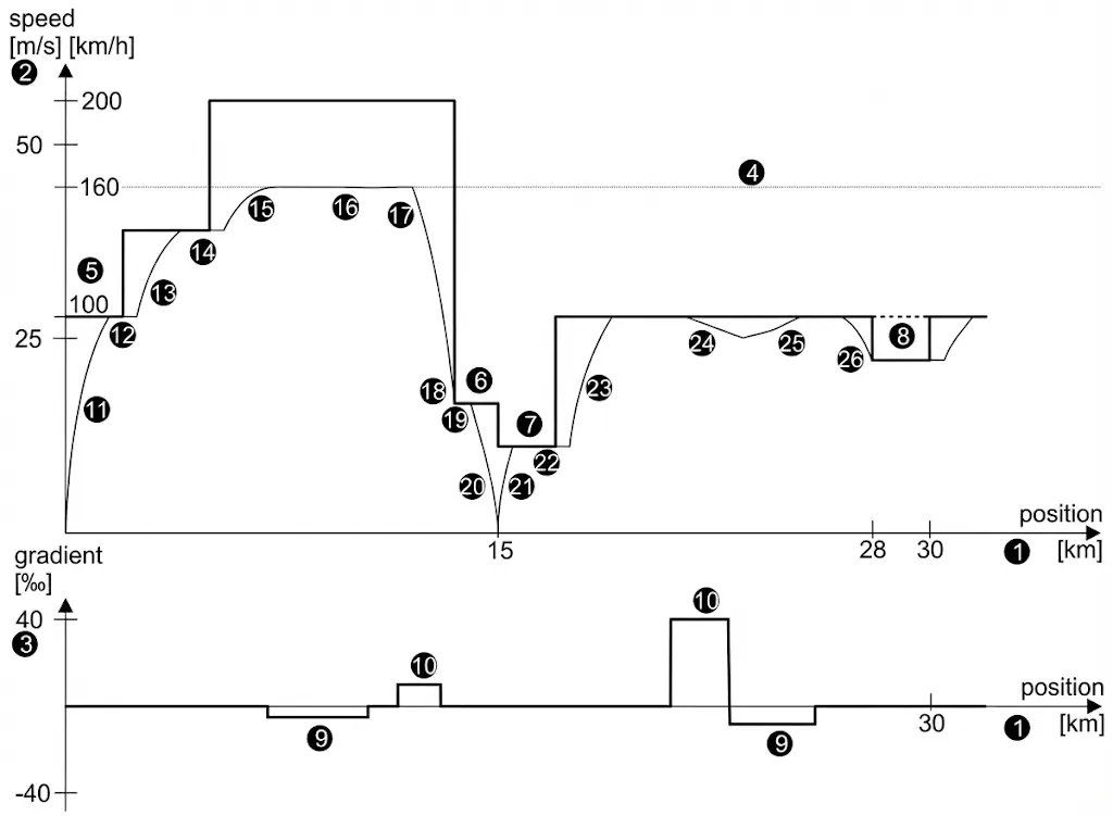
In the represented diagram it is possible to identify following structural elements and technical characteristics:

1. Horizontal axis of diagram represents distance traveled expressed in kilometers.
2. Vertical axis of first graph shows train speed in kilometers per hour, with secondary scale in meters per second.
3. Vertical axis of second subordinate diagram represents layout inclination expressed in thousandths (mm/m), positive values being indicators of ramps (ascents) and negative indicators of gradients (descents).
4. Nominal maximum train speed considered is 160 km/h.
5. Track speed limit presents variations along route, starting at 100 km/h, increasing subsequently to 140 km/h and then to 200 km/h in different segments.
6. At kilometer 15 a railway station is located where regulatory entrance speed is 60 km/h. In this simplification of problem, approach speed is independent of specific track used inside station.
7. Station exit speed is 40 km/h.
8. At kilometer 28 exists a special restriction limiting speed to 80 km/h.
9. In gradient diagram can be identified two sections of downward gradient with inclinations of 5 and 8 thousandths respectively. Depending on available braking capacity, these gradients can impose additional speed restrictions.
10. There exist two sections with upward ramp of 40 thousandths each.
11. In initial phase, train accelerates from zero speed until reaching regulatory speed limit of 100 km/h imposed by track.
12. Once limit reached, train maintains constant speed during a segment.
13. When track speed limitation increases, train accelerates again to new limit of 140 km/h. It is important to note that acceleration begins after limitation point because this limit applies to entirety of train (represented by its head). Driver must wait until train tail has completely passed limitation change point before initiating acceleration.
14. Train travels again at constant speed during next segment.
15. In this section, train accelerates until reaching its nominal speed limit of 160 km/h, which is lower than track speed limit.
16. Movement is maintained again at constant speed.
17. At this point braking process begins. Exact location of this point depends on various factors analyzed subsequently.
18. At entry point to a section where speed must be reduced, train must be traveling at required speed for that new segment. To achieve this, braking start point must be calculated adequately through intersection of deceleration curve with speed profile.
19. Train continues at constant speed during this subsequent segment.
20. Train executes deceleration until reaching stop speed (here scheduled waiting time at station should be included).
21. After stop, train accelerates again to authorized station exit speed.
22. Constant speed is maintained during subsequent segment.
23. Train accelerates again until reaching its nominal speed limit, maintaining then this constant speed.
24. In climbing segment (ramp), train experiences speed decrease because available tractive effort is not sufficient to compensate sum of resistance to motion plus ramp gravitational component. This effect is gradual until reaching stable equilibrium speed.
25. When ramp ends, train can accelerate again.
26. At end of route, train reduces its speed again due to speed limitations imposed by track configuration in that zone.

II.1.1. Acceleration Process

During acceleration segments of a typical journey, train uses entirety of available tractive forces provided by traction motor. Simultaneously, all resistances analyzed previously (resistance to motion, curve resistances, inertial resistances) work against this tractive effort, reducing resulting net acceleration.

A critical aspect of analysis is that both tractive effort and resulting acceleration do not remain constant during process. Tractive effort varies with speed (limited by both power and adhesion), and resistance also varies, mainly as quadratic function of speed. This continuous variability implies that application of classic Newton formulation for constant accelerations would be inappropriate. Problem requires, therefore, being formulated and resolved through differential equations adequately capturing variable nature of these forces.

An additional important consideration is that train cannot be treated as a simple point mass. Train contains inside it significant amount of rotating masses, including wheels, axles, and motor rotors in motorized vehicles. These rotating masses contribute to effective inertia superior to simple mass of rolling stock considered as structure. This additional inertia is captured through introduction of corrective factor termed “fictitious mass”:

\[M^{\prime}=M \cdot f_{p}\]

Factor \(f_p\) presents typical values between 1.10 and 1.30 for motor material (vehicles with propulsion), and between 1.02 and 1.09 for towed material (passive vehicles without propulsion).

Fundamental equation of motion, modified to incorporate fictitious mass, is expressed as:

\[F-R=\frac{P}{g} \cdot \gamma \rightarrow F(v)-R(v)=M^{\prime} \cdot \frac{d v}{d t} \rightarrow F(v)-R(v)=M \cdot f_{p} \cdot \frac{d v}{d t}\]

Assuming train as point object whose mass is concentrated at single point, and performing appropriate mathematical transformations, previous equation can be reformulated:

\[\frac{(F(v)-R(v))}{v}=M \cdot f_{p} \cdot \frac{d v}{d t} \cdot \frac{d t}{d s} \rightarrow \frac{(F(v)-R(v))}{v}=M \cdot f_{p} \cdot \frac{d v}{d s}\]

This differential equation can be transformed additionally to obtain relationships allowing calculation of time and distance required to pass from initial speed to final speed:

\[\frac{d t}{d v}=M \cdot f_{p} \cdot \frac{1}{F(v)-R(v)} \quad \frac{d s}{d v}=v \cdot M \cdot f_{p} \cdot \frac{1}{F(v)-R(v)}\]

Through integration of these differential expressions between initial speed \(v_0\) and final speed \(v_1\), it is possible to obtain time and distance required for transition between these states:

\[t=\int_{v_{0}}^{v_{1}} M \cdot f_{p} \cdot \frac{1}{F(v)-R(v)} \mathrm{d} v \quad s=\int_{v_{0}}^{v_{1}} v \cdot M \cdot f_{p} \cdot \frac{1}{F(v)-R(v)} \mathrm{d} v\]

In operational and engineering practice, these analytical integrals cannot always be solved in closed form. Therefore, numerical approach is adopted dividing total speed interval into multiple sub-intervals (typically of 1 m/s or smaller), calculating for each sub-interval required parameters. Methodology is following:

• Step 1: Average speed of sub-interval is calculated.
• Step 2: Using this average speed, available adherent effort and total resistance are determined.
• Step 3: Difference between tractive effort and resistance provides net force available to accelerate train.
• Step 4: Employing Newton formulation with calculated values, each sub-interval is resolved iteratively.

II.1.2. Acceleration Process: Practical Example

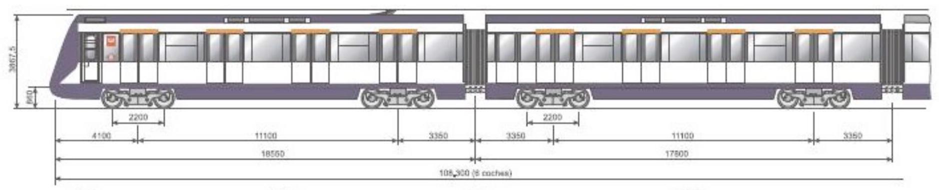
To illustrate application of these concepts, practical case of Madrid Metro 7000 series train is considered, with following technical parameters:

• Total train weight in loaded condition: 298,340 daN
• Driving axles weight (adhesive weight): 207,120 daN
• Total available power: 3168 kW (equivalent to 3,168,000 joules per second)
• Mechanical efficiency at rim: 90% (considering transmission losses)
• Initial adhesion coefficient (train stopped): \(\phi_{0}=0.3\)
• Fictitious inertia factor: \(f_{p}=1.07\)

Specific resistance to motion expression for this type of material is:

\[r_{a}(d a N / t)=1.5+0.01 \cdot v+3 \cdot 10^{-4} \cdot v^{2}\]

Proposed problem consists of determining time necessary for train, starting from rest, to reach 100 km/h, as well as distance traveled during this acceleration.

• Firstly points A and B of effort-speed diagram are calculated:
• Point A: Starting effort
• Point B: Adhesion limit point
• At start:

\[E_{a d h}=P_{a d h} \cdot \phi_{0} \rightarrow 207.120 \cdot 0,3=62.136 d a N\]

• Adhesion limit: intersection of adhesion curves with locomotive power curve

\[\begin{aligned} & E_{a d h}=P_{a d h} \cdot \phi_{v} \rightarrow P_{a d h} \cdot \phi_{0} \cdot \frac{1}{1+0.01 \cdot v} \rightarrow 207.120 \cdot 0,3 \cdot \frac{1}{1+0,01 \cdot v} \\ & F(d a N)=100 \cdot 3,6 \cdot \operatorname{Pot}(\mathrm{~kW}) / \mathrm{v}(\mathrm{~km} / \mathrm{h}) \rightarrow 100 \cdot 3,6 \cdot 3168 \cdot 0,9 / \mathrm{v} \\ & E_{a d h}=F \rightarrow v v_{B}=19,8 \mathrm{~km} / \mathrm{h}=5,5 \mathrm{~m} / \mathrm{s} \end{aligned}\]

Problem Resolution:

First step in resolution is identification of extreme points in effort-speed diagram. Point A corresponds to starting condition (zero speed), where effort limited by adhesion is maximum. Point B represents limit between region controlled by adhesion and region controlled by power.

Calculation of Starting Effort (Point A):

\[E_{a d h}=P_{a d h} \cdot \phi_{0} \rightarrow 207.120 \cdot 0.3=62.136 \text{ daN}\]

Determination of Adhesion Limit Point (Point B):

Point B is identified where adhesion and power curves intersect. At this point:

\[E_{a d h}=P_{a d h} \cdot \phi_{0} \cdot \frac{1}{1+0.01 \cdot v} = F(daN)=100 \cdot 3.6 \cdot Pot(kW) / v(km/h)\]

Solving this equation yields: \(v_B = 19.8 \text{ km/h} = 5.5 \text{ m/s}\)

Numerical Discretization of Acceleration Process (Adhesion Control Phase):

Process is discretized in 1 m/s intervals from point A (v=0) to point B (v=19.8 km/h). As illustrative example, calculation of first sub-interval (from 0 to 1 m/s) is developed:

\[\begin{aligned} E_{adh} &= 207.120 \cdot 0.3 \cdot \frac{1}{1+0.01 \cdot 1.8}\\ R &= (1.5+0.01 \cdot 1.8+3 \cdot 10^{-4} \cdot 1.8^{2}) \cdot 298.340 \cdot 10 / 9.8\\ F_{util} &= E_{adh} - R = 60.575 \text{ daN}\\ a &= \frac{F_{util} \cdot 10}{M \cdot f_p} = 1.860 \text{ m/s}^2\\ t &= \frac{\Delta v}{a} = 0.54 \text{ s}\\ l &= v_0 \cdot t + \frac{1}{2} \cdot a \cdot t^2 = 0.27 \text{ m}\\ Energy &= E_{adh} \cdot l = 164,113 \text{ N·m} \end{aligned}\]

Adhesion Control Phase (Cumulative Table):

Calculations for complete interval from zero speed to point B are presented in following table:

Init. Vel (m/s)	Final Vel (m/s)	Avg. Vel (m/s)	Avg. Vel (km/h)	Adh. Eff. (daN)	Resist. (daN)	Util. Eff. (daN)	Accel. (m/s²)	Time (s)	Distance (m)
0	1	0.5	1.8	61037	462.4	60575	1.860	0.54	0.27
1	2	1.5	5.4	58953	475.7	58477	1.795	0.56	0.84
2	3	2.5	9	57006	491.4	56514	1.735	0.58	1.44
3	4	3.5	12.6	55183	509.5	54673	1.678	0.60	2.09
4	5.5	4.75	17.1	53062	535.4	52527	1.613	0.93	4.42
PHASE I TOTALS								3.20	9.05

Transition to Power Control Phase:

From speed of point B (5.5 m/s or 19.8 km/h), limitation changes from adhesion to power. To verify final speed of 100 km/h is reachable, condition \(F \geq R\) is verified:

\[F(daN) = 100 \cdot 3.6 \cdot Pot(kW) / v(km/h) = 100 \cdot 3.6 \cdot 3168 \cdot 0.9 / 100 = 10,263 \text{ daN}\] \[R = (1.5+0.01 \cdot 100+3 \cdot 10^{-4} \cdot 100^{2}) \cdot 298.340 \cdot 10 / 9.8 = 1,674.5 \text{ daN}\]

As \(F > R\), speed of 100 km/h is reachable. Proceeding then with new table replacing adhesion limited effort with power limited effort:

Init. Vel (m/s)	Final Vel (m/s)	Avg. Vel (m/s)	Avg. Vel (km/h)	Trac. Eff. (daN)	Resist. (daN)	Util. Eff. (daN)	Accel. (m/s²)	Time (s)	Distance (m)	Energy (N·m)
5.5	10	7.75	27.9	36790	612.7	36177	1.111	4.05	31.40	1,155,252

v0 \(\mathrm{m} / \mathrm{s}\)	v1 \(\mathrm{m} / \mathrm{s}\)	vavg \(\mathrm{m} / \mathrm{s}\)	vavg km/h	Ftrac daN	Resist daN	Futil daN	acceleration m/s2	time s	length m	Energy N.m
5.5	10	7.75	27.9	36790	612.7	36177	1.111	4.05	31.40	1155252
10	15	12.5	45	22810	778.6	22031	0.676	7.39	92.41	2107814
15	20	17.5	63	16293	1010.9	15282	0.469	10.66	186.51	3038760
20	25	22.5	81	12672	1302.4	11370	0.349	14.33	322.31	4084351
25	27.78	26.39	95.004	10804	1570.2	9234	0.283	9.81	258.80	2796118
Total								46.23	891.44	13182296

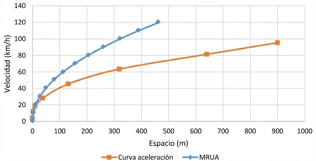
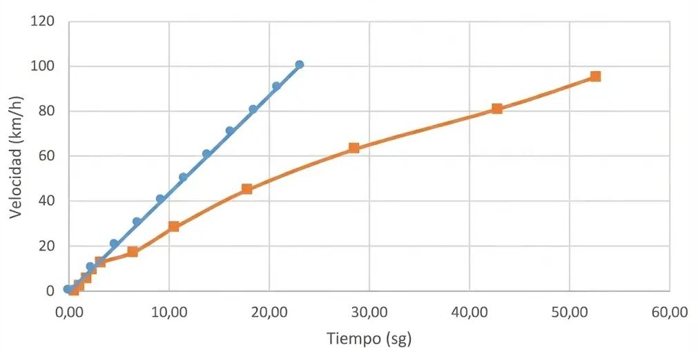
• Therefore, train reaches \(100 \mathrm{~km} / \mathrm{h}\) in 49 sec and travels 892 meters.

v0 m/s	v1 m/s	vavg m/s	vavg km/h	Fadh daN	Resist daN	Futil daN	a m/s2	time s	length m
0	1	0.5	1.8	61037	462.4	60575	1.860	0.54	0.27
1	2	1.5	5.4	58953	475.7	58477	1.795	0.56	0.84
2	3	2.5	9	57006	491.4	56514	1.735	0.58	1.44
3	4	3.5	12.6	55183	509.5	54673	1.678	0.60	2.09
4	5.5	4.75	17.1	53062	535.4	52527	1.613	0.93	4.42
						Total		3.20	9.05

v0 \(\mathrm{m} / \mathrm{s}\)	v1 \(\mathrm{m} / \mathrm{s}\)	vavg \(\mathrm{m} / \mathrm{s}\)	vavg km/h	Ftrac daN	Resist daN	Futil daN	acceleration m/s2	time s	length m
5.5	10	7.75	27.9	36790	612.7	36177	1.111	4.05	31.40
10	15	12.5	45	22810	778.6	22031	0.676	7.39	92.41
15	20	17.5	63	16293	1010.9	15282	0.469	10.66	186.51
20	25	22.5	81	12672	1302.4	11370	0.349	14.33	322.31
25	27.78	26.39	95.004	10804	1570.2	9234	0.283	9.81	258.80
Total								46.23	891.44

Speed Profile

II.1.3. Movement at Constant Speed

When a train has reached its operational limit speed established by track or rolling stock restrictions, and accesses a segment where it can maintain this speed, movement is characterized by zero acceleration. Under these conditions, direct application of classic Newton laws is valid, provided available tractive effort minus resistances remains at positive or zero value. Fundamental relationship for movement at constant speed is:

\[s=v \cdot t\]

However, important practical considerations exist in certain scenarios. When train enters a steep ramp, resistances can increase significantly (sum of resistance to motion plus gravitational component). Under these circumstances, available effort might be insufficient to maintain speed, resulting in deceleration. In such case, section must be analyzed as acceleration section with negative magnitude (deceleration). Conversely, in sections with significant downward gradient, train tends to accelerate under influence of favorable gravitational component. To maintain maximum authorized speed, it is frequently necessary to employ braking systems continuously or modulated. In certain simplified analyses, movement at nominally constant speed is approximated as alternating succession of brief accelerations and coasting segments without active propulsion.

II.1.4. Braking Process

In simplified analysis of braking with constant deceleration, direct analytical equations can be employed. Under hypothesis of constant deceleration \(\gamma\) during braking maneuver, distance required to decelerate from initial speed \(v_0\) to stop is:

\[s=\frac{1}{2} \cdot \frac{v_{0}^{2}}{\gamma}\]

In practical railway operation, deceleration values \(\gamma\) used in calculations are predetermined for different braking types, considering passenger comfort and technical capability of available braking systems:

• Suburban trains (standard braking): \(\gamma = 0.525 \text{ m/s}^2\)
• Long distance passenger trains (comfortable braking): \(\gamma = 0.375 \text{ m/s}^2\)
• Freight trains (conservative braking): \(\gamma = 0.225 \text{ m/s}^2\)

For correct dimensioning of speed profiles on a route, it is essential to know maximum permitted speed on subsequent line segment. This future speed determines maximum exit speed permitted in current section, influencing required braking maneuvers.

Braking distance necessary to transition from maximum speed of current section to maximum speed of next section is calculated by:

\[s_{b}=\frac{v_{\max }^{2}}{2 \cdot \gamma}-\frac{v_{exit}^{2}}{2 \cdot \gamma}\]

Operational Cases in Braking:

If required braking distance \(s_b\) is less than total length of section, then section can be decomposed into two parts: first part circulating at constant maximum speed, followed by second part applying braking curve from \(v_{max}\) to \(v_{exit}\), with exact length of \(s_b\).

If, on the contrary, braking distance \(s_b\) is equal to or greater than total length of section \(s_{sec}\), then it is not possible to maintain maximum speed during section. In this case, maximum entry speed to section \(v_{entr}\) must be determined allowing reaching required exit speed respecting deceleration limits:

\[v_{entr}=\sqrt{2 \cdot \gamma \cdot s_{sec}+v_{exit}^{2}}\]

It is important to highlight that if maximum permitted speed in current section \(v_{max}\) turns out to be greater than calculated entry speed \(v_{entr}\), then maximum exit speed of previous section must be equaled to \(v_{entr}\).

Due to these interdependencies, it is standard practice in railway engineering to determine braking profiles working in reverse order to travel direction: initiating from last section of route and advancing progressively backwards. This approach ensures upstream restrictions adjust correctly to downstream requirements.

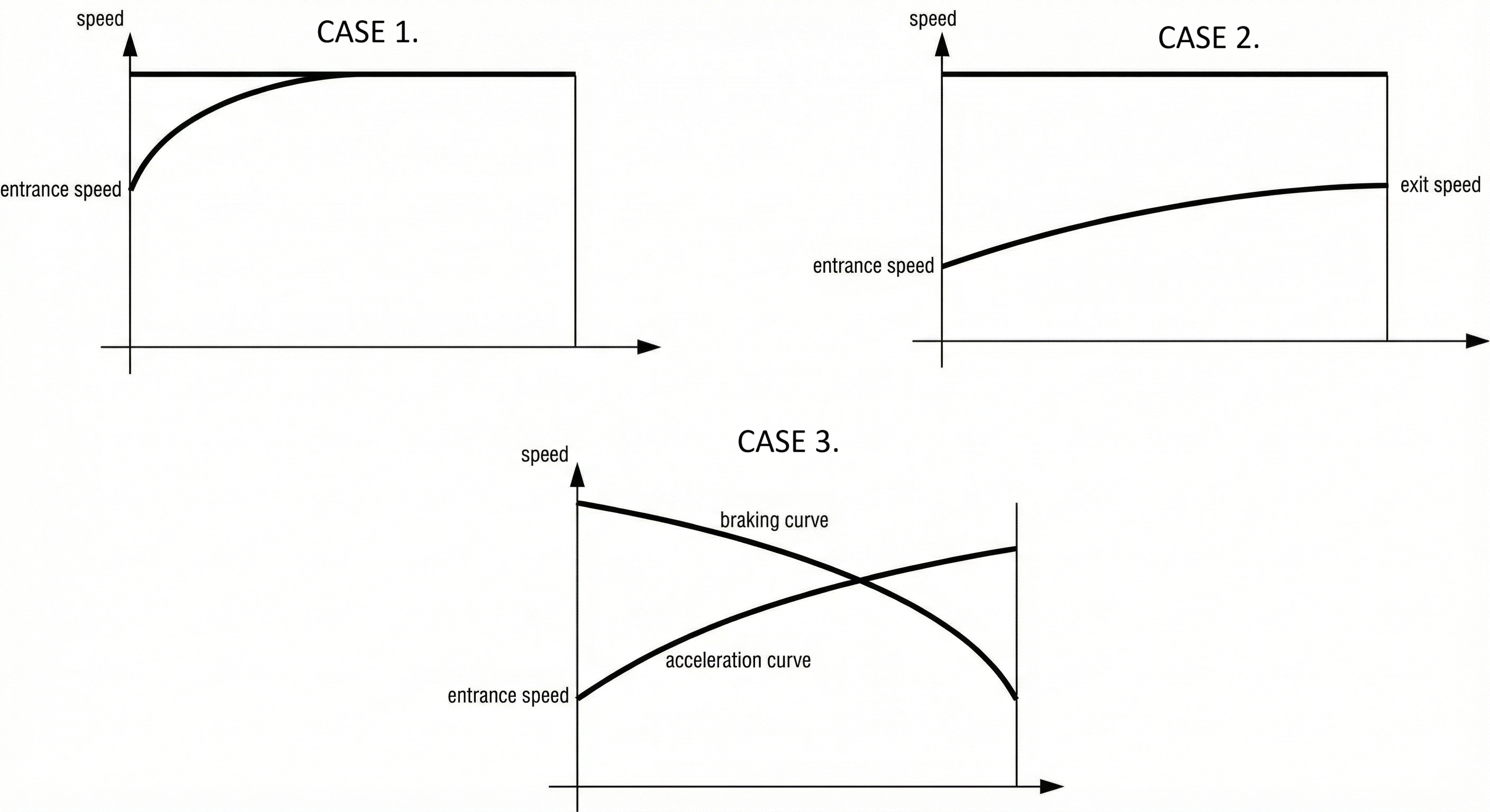
CASE 1: Section with constant maximum speed reached in said section

In this operational scenario, considered line section is sufficiently long for train to accelerate from entry speed and reach maximum permitted speed, maintaining it subsequently during a portion of segment. Speed profile in this case consists of three phases: acceleration from \(v_{entry}\) to \(v_{max}\), movement at constant speed \(v_{max}\), and finally braking from \(v_{max}\) to \(v_{exit}\).

CASE 2: Exit speed lower than maximum; acceleration distance superior to section length

In this case, line section is not sufficiently long to allow train to reach its maximum speed. This occurs when distance required to accelerate from entry speed to maximum speed exceeds total available length of section. As result, train accelerates continuously during entire section without reaching maximum speed, arriving at intermediate exit speed lower than \(v_{max}\).

CASE 3: Braking section with curve intersection

In this scenario, section constitutes primarily a braking segment. Train enters section with certain speed and must reduce its speed to comply with maximum speed requirements of next section. Acceleration/deceleration curves intersect within section, meaning train executes modulated braking maneuver to reach required speed exactly at transition point with next section.

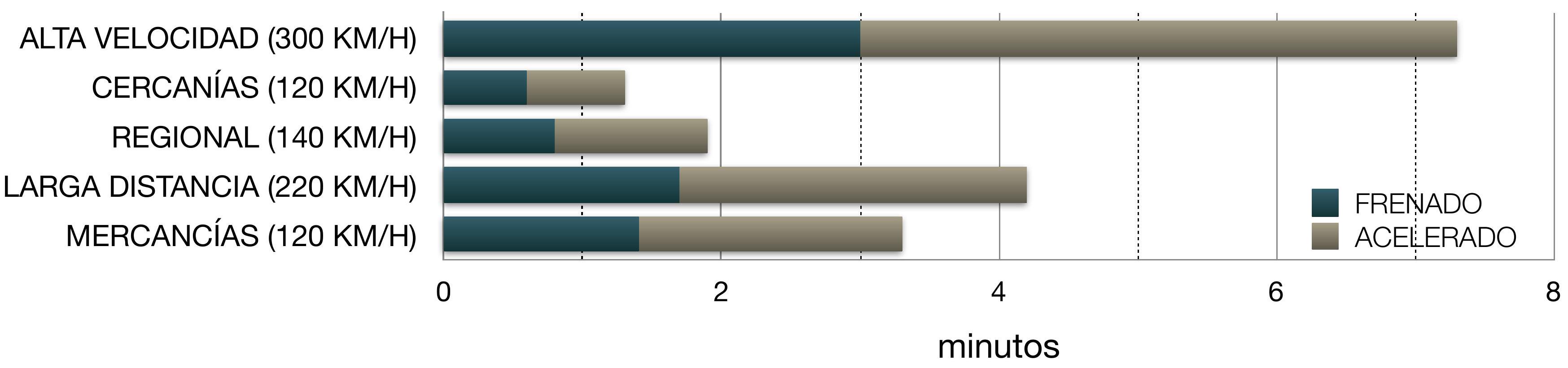
Time necessary to accelerate and brake (minutes)

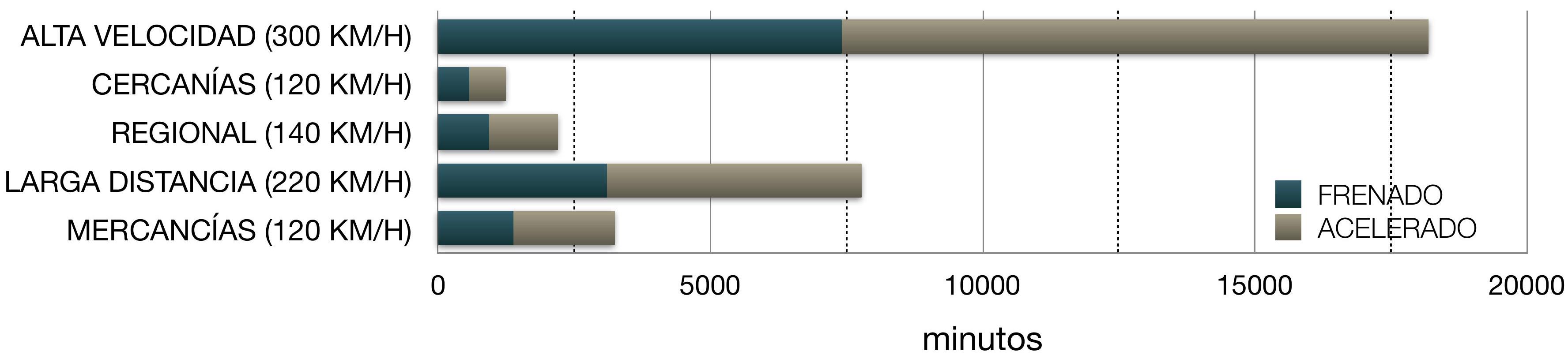
Distance necessary to accelerate and brake (meters)

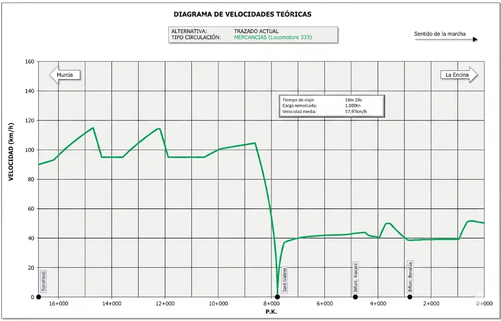
II.2. Maximum Speeds

Chapter III Travel Time Calculation - Base run

“Base run” constitutes fundamental concept in railway planning and operation. It is defined as minimum theoretically possible time to traverse specific section of railway line transporting determined load. This calculation is performed under set of standard conditions representing nominal and reliable operation. Specifically, base run incorporates:

• Optimal train driving by driver, assuming professional and standardized handling
• Intrinsic technical performance of motor material employed
• Characteristics of traction energy supply system (voltage, current, etc.)
• Adhesion capacity between wheels and rail under normal conditions
• Resistance to motion presented by both towed material and infrastructure (ramps, curves, etc.)
• Speed limits permitted by geometric layout and infrastructure

Base run calculation is absolutely indispensable for schedule design and railway service programming. To obtain precise calculations it is necessary to have detailed information of maximum speeds permitted in each line section, information which in turn determines travel times required in each section.

III.1. Standard Run

According to UIC 451-1 (2000) specification sheet, concept of “Standard Run Time” is defined as temporal interval required between two determined points to establish operational schedule of a train. This parameter constitutes sum of three critical components: time derived from base run calculation, added with regularity margins and supplementary margins incorporated according to line operational requirements.

Simula FFCC

Regularity margin constitutes additional time incorporated into previously calculated base travel time, with purpose of systematically compensating operational delays originating from various causes. These include periodic maintenance tasks of railway facilities, which although plannable, require operational modulation. Likewise, possible lost times derived from operational technical incidents, unfavorable weather conditions, or prolonged station stops due to passenger influx saturation are contemplated.

Supplementary margin, in contrast, represents temporal increase reserved specifically to compensate delays caused by major works on installations during prolonged periods. This margin also incorporates delays occurring systematically in large complex railway nodes, mainly caused by extensive shunting operations resulting from available infrastructure configuration and complexity.

Regularity Margin:

A) NON-SELF-PROPELLED PASSENGER TRAINS

• A minimum of 1.5 minutes \(/ 100 \mathrm{~km}\) increased based on following criterion V. limit \(\leq 140 \mathrm{~km} / \mathrm{h} \quad 141-160 \mathrm{~km} / \mathrm{h} \quad 161-200 \mathrm{~km} / \mathrm{h} \quad>200 \mathrm{~km} / \mathrm{h}\) Tonnage

\(\leq 300 \mathrm{t}\)	3%	3%	4%	5%
301-500 t	4%	4%	5%	%
501-700 t	4%	5%	6%	%
\(>700 \mathrm{t}\)	5%	5%	6%	7%

• A minimum of at least 3.5 minutes \(/ 100 \mathrm{~km}\)

B) SELF-PROPELLED PASSENGER TRAINS

• A minimum of 1 minute per 100 km, increased according to specific criteria depending on maximum operating speed. This structure allows faster trains to have additional temporal margins to maintain their operational regularity.

In high-speed systems where only self-propelled units circulate, regulatory flexibility is permitted: supplementary percentage regarding travel time can oscillate between 3% and 7% for speeds exceeding 200 km/h, allowing optimization according to specific characteristics of each line and service.

C) FREIGHT TRAINS

Calculation of regularity margins for freight trains presents differentiated structure according to operating speed range. For speeds up to 120 km/h, operational flexibility is offered with three equivalent alternatives available: margin of 1 minute per 100 km increased to 3%, fixed margin of 3 minutes per 100 km, or global percentage of 4%. This multiplicity of options allows operators to select criterion best adapting to their specific operating conditions. For speeds exceeding 120 km/h, freight trains are governed by same criteria established for non-self-propelled passenger trains, thus assimilating fast freight trains to passenger transport standards. Resulting calculation is expressed as: 1 minute per 100 km plus percentage X of base run time.

Supplementary margin differs fundamentally from regularity margin both in nature and calculation. Unlike latter, it is not calculated as percentage of travel time but as fixed temporal interval applied to each specific line section considered. When this margin is due to operational complexity of important railway node, it is recommended not to exceed 3 minutes to maintain system efficiency. Its application is strictly limited to non-habitual operating circumstances, preserving its character as exception mechanism for exceptional operational situations.

Scheduled waiting times constitute additions to travel time incorporated for superior operational coordination reasons. These times are added to conveniently synchronize schedules of different passenger lines at modal interchange nodal points, to coordinate programming of multiple expeditions within integrated master schedule, or to allow operational maneuvers like crossings and overtakings in specific track sections within section.

III.2. Schedule/Itinerary Book

III.3. Calculation of Consumed Energy

Evaluation of energy consumption in trains during their movement can be approached through two complementary methodologies, each with specific purposes and applications. First approach consists of instantaneously integrating energy consumption under each specific operational condition: movement at uniform speed in horizontal sections, behavior in ascents and descents, transient processes of speed reduction and increase, among others. This method results especially valuable for “instantaneous” operational decision making such as optimization of economic driving or controlled energy return to distribution grid, although it has limitation that it does not explicitly reveal underlying causes of observed consumption.

Second approach examines integral energy balance of train considering entirety of a determined route, typically calculated between two points where train is at rest and at same altitude. This methodology results particularly useful for global scope calculations such as infrastructure design, specification of new railway vehicles, or service schedule programming. Its fundamental advantage lies in allowing disaggregating and making explicit specific causes of energy consumption: what portion is attributed to curves, what part to tunnels, how much energy is dissipated by air intake and aerodynamic resistances, etc.

III.4. Introduction

To illustrate instantaneous energy calculation approach, consider previous acceleration analysis example. Energy consumption is obtained multiplying tractive force applied in each interval by distance traveled during that interval. Following two tables present detailed breakdown of energy consumption during two distinct acceleration phases:

v0 \(\mathrm{m} / \mathrm{s}\)	v1 \(\mathrm{m} / \mathrm{s}\)	vavg \(\mathrm{m} / \mathrm{s}\)	vavg km/h	Fadh daN	Resist daN	Futil daN	a m/s2	time s	length m	Energy \(\mathrm{N} \cdot \mathrm{m}\)
0	1	0.5	1.8	61037	462.4	60575	1.860	0.54	0.27	164113
1	2	1.5	5.4	58953	475.7	58477	1.795	0.56	0.84	492583
2	3	2.5	9	57006	491.4	56514	1.735	0.58	1.44	821428
3	4	3.5	12.6	55183	509.5	54673	1.678	0.60	2.09	1150709
4	5.5	4.75	17.1	53062	535.4	52527	1.613	0.93	4.42	2344544
Total								3.20	9.05	4973377

v0 \(\mathrm{m} / \mathrm{s}\)	v1 \(\mathrm{m} / \mathrm{s}\)	vavg \(\mathrm{m} / \mathrm{s}\)	vavg km/h	Ftrac daN	Resist daN	Futil daN	acceleration m/s2	time s	length m	Energy \(\mathrm{N} \cdot \mathrm{m}\)
5.5	10	7.75	27.9	36790	612.7	36177	1.111	4.05	31.40	11552520
10	15	12.5	45	22810	778.6	22031	0.676	7.39	92.41	21078135
15	20	17.5	63	16293	1010.9	15282	0.469	10.66	186.51	30387605
20	25	22.5	81	12672	1302.4	11370	0.349	14.33	322.31	40843513
25	27.78	26.39	95.004	10804	1570.2	9234	0.283	9.81	258.80	27961182
Total								46.23	891.44	131822956

According to this, traction energy consumed in journey is 136.8 •106 \(\mathrm{N} \cdot \mathrm{m}\), that is 38 kWh.

Energy to accelerate train can proceed:

• from traction motor
• from potential energy loss (when descending a gradient).

When kinetic energy is reduced (train is decelerated) energy can be employed:

• overcoming resistance to motion;
• climbing a ramp;
• dissipated in brake (this is what is truly lost).

If train could store energy without restrictions, energy consumption at rim would be only necessary to overcome resistance to motion, because:

• All energy consumed to accelerate train would be stored when reducing speed.
• Entirety of \(E_{\text {pot }}\) received in ascents could be recovered in descents: there would be no net external energy consumption for this concept.

If it could not store, nor use any of \(E_{\text {cin }}\) nor \(E_{\text {pot }}\), train energy consumption would be:

• energy to overcome resistance to motion \(\left(R_{\text {av }}\right)+\)
• energy to accelerate it all times it must increase its \(V+\)
• energy to climb all ramps of route.

Indirect knowledge of energy entered into train is obtained through application of fundamental principle of energy conservation. Basic formulation establishes that energy entering system is equivalent to sum of energy exiting it, plus energy accumulating inside train in form of gravitational or kinetic potential, considering also losses inherent to performance of mechanical and electrical systems.

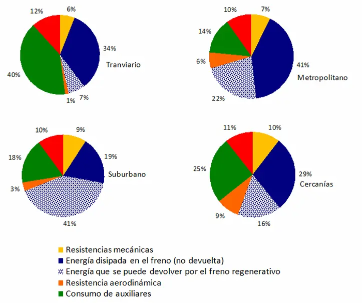
Energy exiting train decomposes into three main categories: employed to overcome resistance to motion during entire section (including mechanical resistance components by curves, resistance associated to air intake in vehicle, and aerodynamic pressure and friction resistances); dissipated or regenerated through braking system, which can be employed to decelerate train in stops or speed reduction points, or to prevent unwanted acceleration on very steep gradients; and finally consumed by train auxiliary services (climate control, lighting, control systems, etc.).

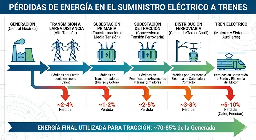
To obtain final energy required at pantograph or charging point, it is necessary to incorporate to vehicle useful consumptions losses associated to locomotive and auxiliary equipment performance. Subsequently, considering losses in electrical energy transport and conversion processes in substations, total electrical energy to be purchased from system is obtained. Finally, incorporating losses inherent to production processes of energy vector in generating plants, quantification of primary energy consumed is reached, representing total resource consumption associated to train movement.

III.5. Transport and Conversion Losses

III.6. Energy Exiting the Train

Energy by Mechanical Resistance to Motion

• on straight: \(\begin{aligned} & E_{\text {rMotion } R}(k W h)=A(d a N) \cdot L\left(k m_{\text {line }}\right) \cdot \frac{1}{360} \\ & \text { where: } \quad A(d a N)=\left(M_{\text {load }}(t) \cdot 0.25\right)+\left(N_{\text {axles }} \cdot 7\right) \end{aligned}\)

• on curves of radius R:

\[E_{r Motion Curve}(k W h)=L\left(k m_{line}\right) \cdot M(t) \cdot a_{cur} \cdot \frac{1}{360}\]

where:

\[a_{c u r}(d a N / t)=\frac{1}{L_{l i n e}(m)} \cdot \sum_{c}\left(l_{c}(m) \cdot \frac{600 or 800}{R_{c}(m)}\right)\]

Length of section considered (m)
Radius(m)	Length(m)	Acc. Len (m)	Curve Coef.
1.076	300	251	447.21
863	100	201	349.02
690	600	216	897.39
500	250	258	919.20

Energy by Air Intake

Air circulation through train climate control and ventilation systems generates additional resistance that must be overcome during movement. This energy consumption is proportional both to volume of processed air and train circulation speed. Required energy is expressed by:

\[E_{\text{airintake}}(kWh)=B(daN/km/h) \cdot V(km/h) \cdot L_{\text{line}}(km) \cdot \frac{1}{360}\]

where coefficient B is determined by:

\[B(daN/km/h)=Q(m^{3}/s) \cdot \rho \cdot \frac{1}{36} \approx 0.034 \cdot Q(m^{3}/s)\]

Practical Example: Train 103 Madrid-Barcelona

Consider case of Madrid-Barcelona high speed traction service, presenting total energy consumption of approximately 11,561 kWh. In this route, air intake system (with volumetric flow of 99.70 m³/s) assumes energy consumed of:

\[3.39 \text{ daN}/(km/h) \times 198 \text{ km/h} \times 620 \text{ km} \times 1/360 = 2.264 \text{ kWh (19.58%)}\]

This result evidences that aerodynamic resistance by air intake represents approximately 10% of total consumption in this specific service.

Aerodynamic Energy Exiting Train.

\[E_{\text {aOpen }}(k W h)=C\left(d a N /(k m / h)^{2}\right) \cdot\left(V_{\text {avg }}^{2}+\sigma(V)^{2}\right)(k m / h)^{2} \cdot L_{\text {line }}(k m) \cdot \frac{1}{360}\]

where:

\[C\left(d a N /(k m / h)^{2}\right) \cong c_{p} \cdot S_{f}\left(m^{2}\right)+c_{f} \cdot p_{wet}(m) \cdot L_{train}(m)\]

Energy to overcome additional aerodynamic resistance in tunnel:

\[E_{\text {tunnel }}=E_{\text {open }}(k W h) \cdot \frac{L_{\text {tunnel }}}{L_{\text {line }}} \cdot\left(T_{f}-1\right)\]

	\(\mathrm{C}_{\mathrm{p}}\)	\(\mathrm{C}_{\mathrm{f}}\)
HS	0.00096	0.000021
Conventional	0.0022	0.0003

Energy to overcome aerodynamic resistance due to outside wind

When train moves in significant side or head wind conditions, aerodynamic resistance increases proportionally to square of relative speed between train and surrounding air. This additional energy must be supplied by traction system to maintain scheduled operational speed. Formulation is:

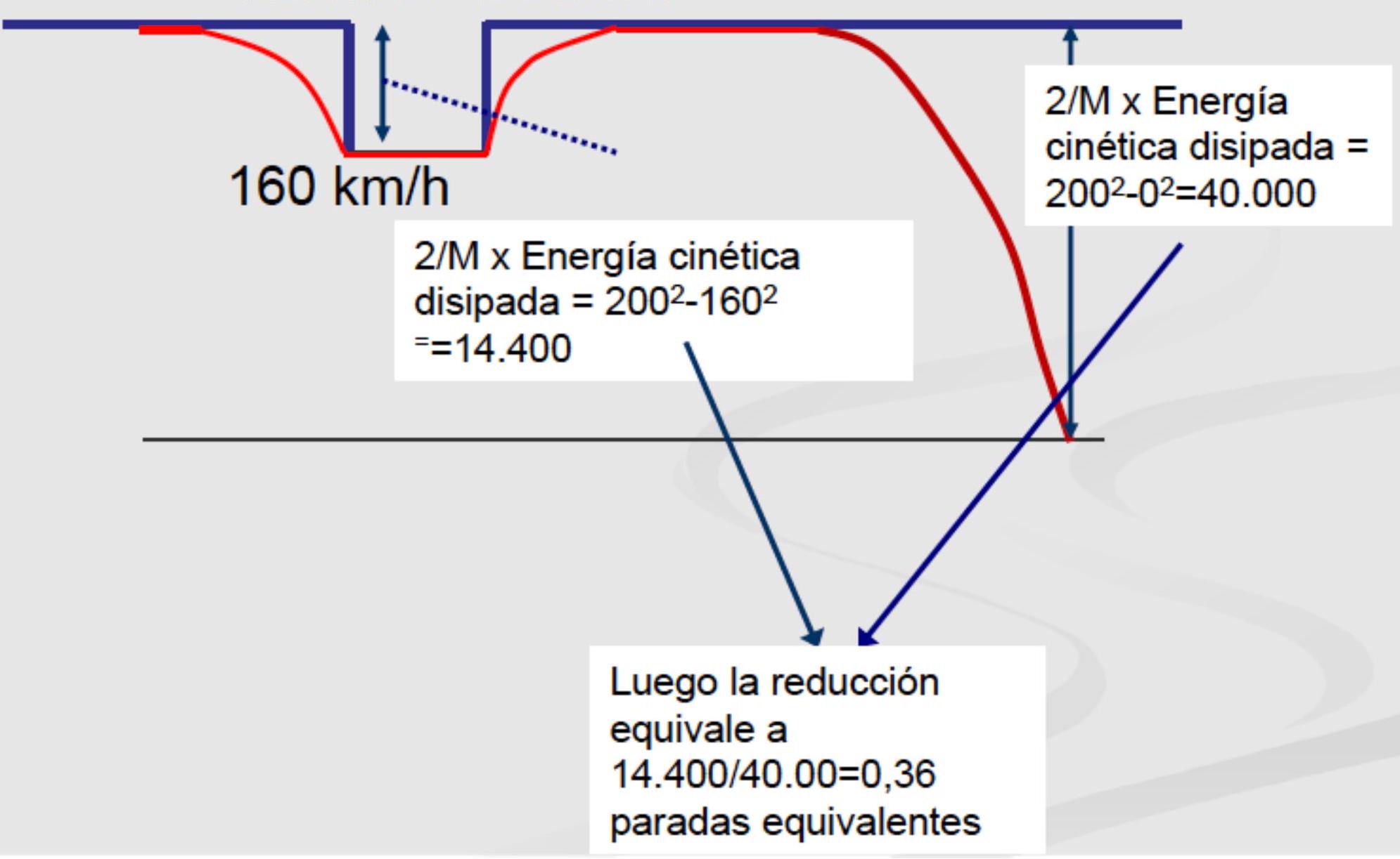
\[E_{\text{wind}}=C \cdot (V_{\text{wind}} \cdot 0.43)^{2} \cdot L_{\text{line}}(km) \cdot \frac{1}{360}\]

Kinetic energy dissipated in speed reductions from Vop to 0km/h \(E_{cinRedV}(kWh) = N_{stops} \cdot 0.5 \cdot (M_{load} + M_{rot}) \cdot V_{op}^{2} \cdot \frac{1}{3.6^{2} \cdot 10^{3}}\) It must also be considered energy that must be subtracted from balance: that which was originally consumed to overcome resistance to motion during deceleration segments before each stop. This energy is theoretically recoverable through regenerative braking systems, but in practice partially dissipates in mechanical braking system. Quantification is:

\[E_{\text{ravd}}(kWh)=N_{\text{stops}} \cdot \left[\frac{A \cdot V_{op}^{2}}{2 \cdot \gamma}+\frac{B \cdot V_{op}^{3}}{3 \cdot \gamma}+\frac{C \cdot V_{op}^{4}}{4 \cdot \gamma}\right] \cdot \frac{1}{3.6^{3} \cdot 10^{5}}\]

Equivalent Stops and Speed Reductions

Within energy consumption analysis, not only commercial stops (at stations) and technical (for maintenance) count, but also all those speed reductions caused by maximum speed limitations of line profile. Each speed reduction not corresponding to commercial or technical stop is counted as “fraction of stop” with energetic equivalence. Total calculation of equivalent stops for energy consumption purposes is:

\[N^{\circ}_{\text{equiv stops}} = N^{\circ}_{\text{commercial stops}} + 1_{\text{(final stop)}} + N^{\circ}_{\text{technical stops}} + \sum_{\text{reductions}} \text{fractions of equivalent stops}\]

This analysis allows disaggregating total consumption between stations: what energy is consumed in accelerating from stop, what energy is dissipated in brakings, and what energy represents circulation in constant speed sections.

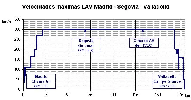
Max. Vel \(200 \mathrm{~km} / \mathrm{h}\)

	km	Speeds N (max 300km/h)	Reductions (max300km/h)
Madrid P. Atocha	0.000	30	0.0000
	1.000	60	0.0000
	1.500	90	0.0000
	2.800	100	0.0000
	4.400	140	0.0000
	5.700	200	0.0000
	13.100	230	0.0000
	20.300	270	0.0000
	99.300	290	0.0000
	103.400	300	0.0000
	112.000	290	0.0656
	115.100	270	0.1244
	170.200	190	0.4089
Ciudad Real	170.500	190	0.0000
	173.100	240	0.0000
	178.100	270	0.0000
	206.800	200	0.3656
	208.800	80	0.3733
Puertollano	209.400	70	0.0167

Equivalent stops by speed reduction = 1.3544 Equivalent commercial stops = 0.4556

• Potential energy dissipated by brake on gradients:

\[E_{\text {potF }}(k W h)=M_{\text {load }}(t) \cdot 9.81 \cdot \text { excGradient } \cdot L(k m) \cdot \frac{1}{3600}\]

• Equilibrium Gradient: For a speed is that in which gravity force equals (in absolute value) resistive force and train is in equilibrium.

\[\text { excGradient }=\frac{\sum\left(p_{\text {real }}-\text { pequilibrium }\right) \cdot l_{\text {gradient }}}{L_{\text {line }}}\]

• If previous value is positive, it is excess gradient. If negative, 0 is taken as excess gradient (no braking)

• Kinetic energy dissipated by brake on gradients:

	(1) If \(\mathrm{p}<\mathrm{pe}_{\mathrm{V}_{\text {max }}}=\mathrm{a}+\mathrm{bV}_{\text {max }}+\mathrm{cV}_{\text {max }}^{2}\) It is necessary to provide traction to maintain \(\mathrm{V}_{\text {max }}\)
	\(\text { (2) If } \mathrm{p}=\mathrm{pe}_{\mathrm{V}_{\text {max }}}=\mathrm{a}+\mathrm{bV}_{\text {max }}+\mathrm{cV}_{\text {max }}^{2}\) Maintains \(\mathrm{V}_{\text {max }}\) without traction or braking
	(3) If \(\mathrm{p}>\mathrm{pe}_{\mathrm{V}_{\text {max }}}=\mathrm{a}+\mathrm{bV}_{\text {max }}+\mathrm{cV}_{\text {max }}^{2}\) It is necessary to brake to not exceed \(\mathrm{V}_{\max .} \rightarrow\) Then energy is lost

Equilibrium gradient -9.875

km start	Value (mm)
0.000	\(-1.46\)
0.266	\(-2.99\)
0.505	\(-0.59\)
0.556	\(-8.05\)
0.826	\(-14.02\)
1.113	\(-9.99\)
1.388	\(-10.05\)
1.755	\(-7.71\)
1.815	\(-10.09\)
1.920	\(-12.36\)
1.985	\(-8.83\)
2.472	\(-9.19\)
3.823	\(-1.13\)
4.097	\(-11.99\)
4.546	11.7
5.075	\(-6.14\)
5.756	9.17
6.122	\(-12.46\)
Excess Height (mm/km)

Potential Energy Consumed by Altitude Difference

When start and end points of route are at different altitudes, exists difference in potential energy that must be considered in total energy balance. If origin is lower than destination, train must consume additional energy to gain height; if conversely destination is lower, part of this energy can be recovered through regenerative braking. Consumed (or recoverable) potential energy is calculated as:

\[E_{\text{potExt}}(kWh)=M_{\text{load}}(t) \cdot 9.81 \cdot \text{diffHeights}(m) \cdot \frac{1}{3600}\]

Energy Consumed by Technical Auxiliary Systems

Climate control, lighting, control systems, water pumps, air compressors and other technical equipment of train require continuous electrical power throughout journey. This energy is considered as operation consumption and must be incorporated into total balance. Typical quantification is:

\[E_{\text{auxTech}}=\text{pow}_{\text{AuxTech}} \cdot T_{\text{trip}} \cdot 0.7\]

where factor 0.7 represents operation coefficient contemplating not all auxiliaries operate at maximum power continuously throughout journey.

Energy Consumed by Commercial Services

Commercial services on board train (lighting, climate control, and other passenger services) represent energy consumption varying according to vehicle dimensions and conditioning characteristics. Energy consumed by these services is estimated by:

\[E_{\text{auxcom}}=[0.3 \text{ to } 0.45] \cdot S_{\text{useful}}(m^{2}) \cdot t_{\text{trainon}}(h)\]

A fundamental aspect is that total consumption in determined route decreases significantly with average operating speed. This phenomenon is because although required power is relatively constant, total trip duration reduces drastically with higher speeds, compensating thus additional traction consumption.

Consider practical example: in 300-seat train with characteristic commercial auxiliary consumption of 200 kWh/h. If Madrid-Barcelona route is performed at conventional speed in 5 hours, auxiliary consumption is 200 × 5 + 200 × 0.75 (rotation period) = 1,150 kWh. If same route is performed in high speed with duration of 2.5 hours, consumption descends to 200 × 2.5 + 200 × 0.75 = 650 kWh, representing saving of 500 kWh in commercial services by simple reduction of operation time.

III.7. Example: Madrid-Barcelona High Speed Line

		AVE MPA-BAR 300	AVE MPA-BAR 250	AVE MPA-BAR 120
Line Characteristics
Length	km	621.00	621.00	621.00
Tunnel Length	km	47.45	47.45	47.45
Tunnel Factor (Tf)		1.50	1.50	1.50
Supply Voltage	kV	\(2 \times 25 \mathrm{kV}\) AC	\(2 \times 25 \mathrm{kV}\) AC	\(2 \times 25 \mathrm{kV}\) AC
Altitude Difference (Hd-Ho)	m	0.00	0.00	0.00
Curve Coefficient	daN/t	0.12	0.12	0.12
Specific Gradient Excess	\(\mathrm{mm} / \mathrm{km}\)	1240.97	1824.75	4510.86
Average Outside Wind Speed	km/h	10	10	10
Service Characteristics
Maximum Speed (no stops)	km/h	300.00	250.00	120.00
Travel Time on route	min	158.00	189.60	395.00
Average Speed (no stops)	km/h	235.82	196.52	94.33
% utilization on standard seats	%	0.65	0.65	0.65
Seat and Service Density		1.00	1.00	1.00
Commercial Stops (excluding final)	\(N^{\circ}\)	0.00	0.00	0.00
Equivalent Commercial Stops		1.00	1.00	1.00
Scheduled Technical Stops	\(N^{\circ}\)	0.00	0.00	0.00
Unscheduled Technical Stops	\(N^{\circ}\)	0.10	0.10	0.10
Equivalent Stops by Reduction	\(N^{\circ}\)	0.10	0.00	0.00
Average Commercial Stop Time	min	2.00	2.00	2.00
Stop Origin Speed		258.28	215.24	103.31

Train Designation		s103	s130	s465 (Civia)
Maximum Speed	km/h	350	250	120
Total Train Power	kW	8800	4800	2200
Empty Mass	\(t\)	425	312	157.3
Equivalent Rotating Masses	\(t\)	40.05	15.41	11.01
Operating Voltage	kV	\(2 \times 25 \mathrm{kV}\) AC	\(2 \times 25 \mathrm{kV}\) AC	\(2 \times 25 \mathrm{kV}\) AC
Real Seats	seats	404	298	997
Coefficient A (mechanical resist.)	daN	337.0762	222.6758	126.55
Coefficient B (air intake resist.)	daN/(km/h)	3.7603	2.4039	1.5314
Coefficient C (aerodynamic resist.)	daN/(km/h)2	0.056361	0.0482798	0.021696
Gross Useful Surface	m2	525.09	359.68	254.05
Motor Type	0	Asynchronous AC	Asynchronous AC	Asynchronous AC
Power per electric traction motor	\(k W\)	550	632	320
Service Brake Deceleration	\(\mathrm{m} / \mathrm{s} 2\)	0.54	0.6	0.6
Traction Chain Efficiency	kWhs/kWhe	0.87	0.87	0.87
Auxiliary Efficiency	kWhs/kWhe	0.85	0.85	0.85
Auxiliary Supply Origin		Catenary	Catenary	Catenary
Has Air Conditioning?	boolean	1	1	1
Heat Transmission Coefficient (K)	\(\mathrm{W} / \mathrm{m} 2^{\circ} \mathrm{C}\)	1.6	1.6	1.6
Lighting Consumption	kWh/h m2	0.05	0.05	0.05
Climate Control Consumption	kWh/h m2	0.2	0.2	0.2
Technical Auxiliaries Power	\(k W\)	50	50	50
Loaded Mass	tons	446.008	327.496	209.144

		AVE MPA-BAR 300	AVE MPA-BAR 250	AVE MPA-BAR 120
Direct Final Energy Consumption		s103	s130	s465 (Civia)
Energy to overcome mech. resistance to motion on straight	kWh	581.46	384.12	218.30
Energy to overcome add. resistance to motion on curves	\(k W h\)	88.94	65.31	41.71
Energy to overcome air intake resistance	\(k W h\)	1,529.67	814.91	249.19
Energy to overcome aerodynamic resistance in open air	kWh	6,485.83	3,858.24	399.47
Additional energy to overcome aerodynamic resist. in tunnel	kWh	247.78	147.40	15.26
Additional energy to overcome aerodynamic resist. due to wind	kWh	1.80	1.54	0.69
Kinetic Energy	kWh	416.13	187.27	27.70
Kinetic energy employed in overcoming resistance to motion	kWh	45.41	15.35	0.73
Kinetic energy dissipated in speed reductions (-employed resist. motion) without econ. driving	kWh	370.71	171.92	26.97
Potential energy dissipated in brake on gradients without economic driving	kWh	936.62	1,011.27	1,596.48
Potential energy consumed by diff. altitude between ends	\(k W h\)	0.00	0.00	0.00
Energy consumed by com. aux. (lighting)	kWh	69.14	56.83	83.62
Energy consumed by com. aux. (climate control)	kWh	276.55	227.32	334.50
Energy consumed by technical auxiliaries	\(k W h\)	92.17	110.60	230.42
Energy (useful) consumed at rims and auxiliaries	\(\boldsymbol{k W h}\)	10,680.65	6,849.46	3,196.61
Losses in traction locomotive (by efficiency)	kWh	1,530.53	964.50	380.75
Losses in auxiliary supply	kWh	77.27	69.66	114.45
Energy (final) imported at pantograph (or diesel inlet)	kWh	12,288.45	7,883.61	3,691.80

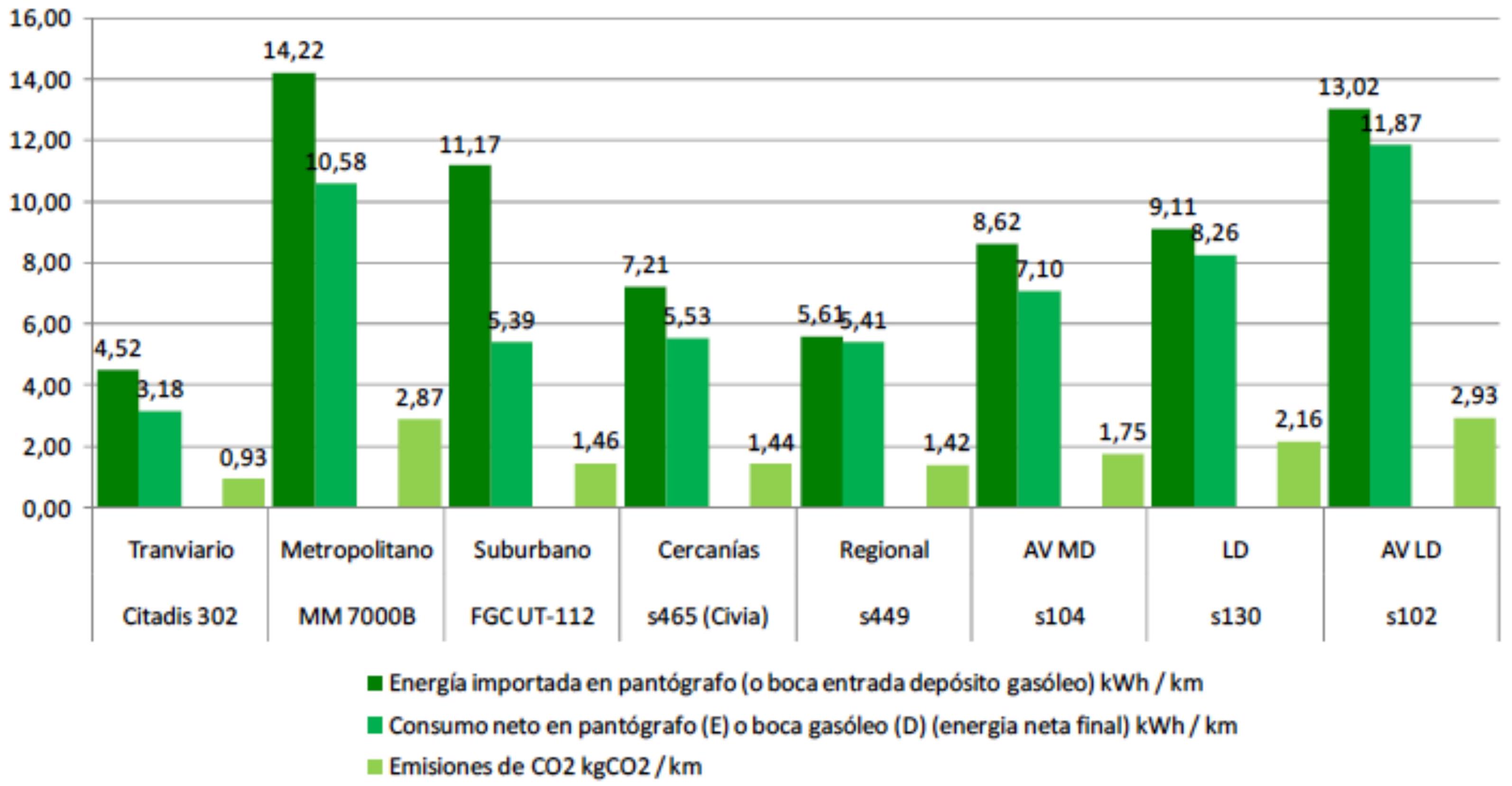
III.8. Energy Consumption

Consumption and Emissions per Train and Kilometer

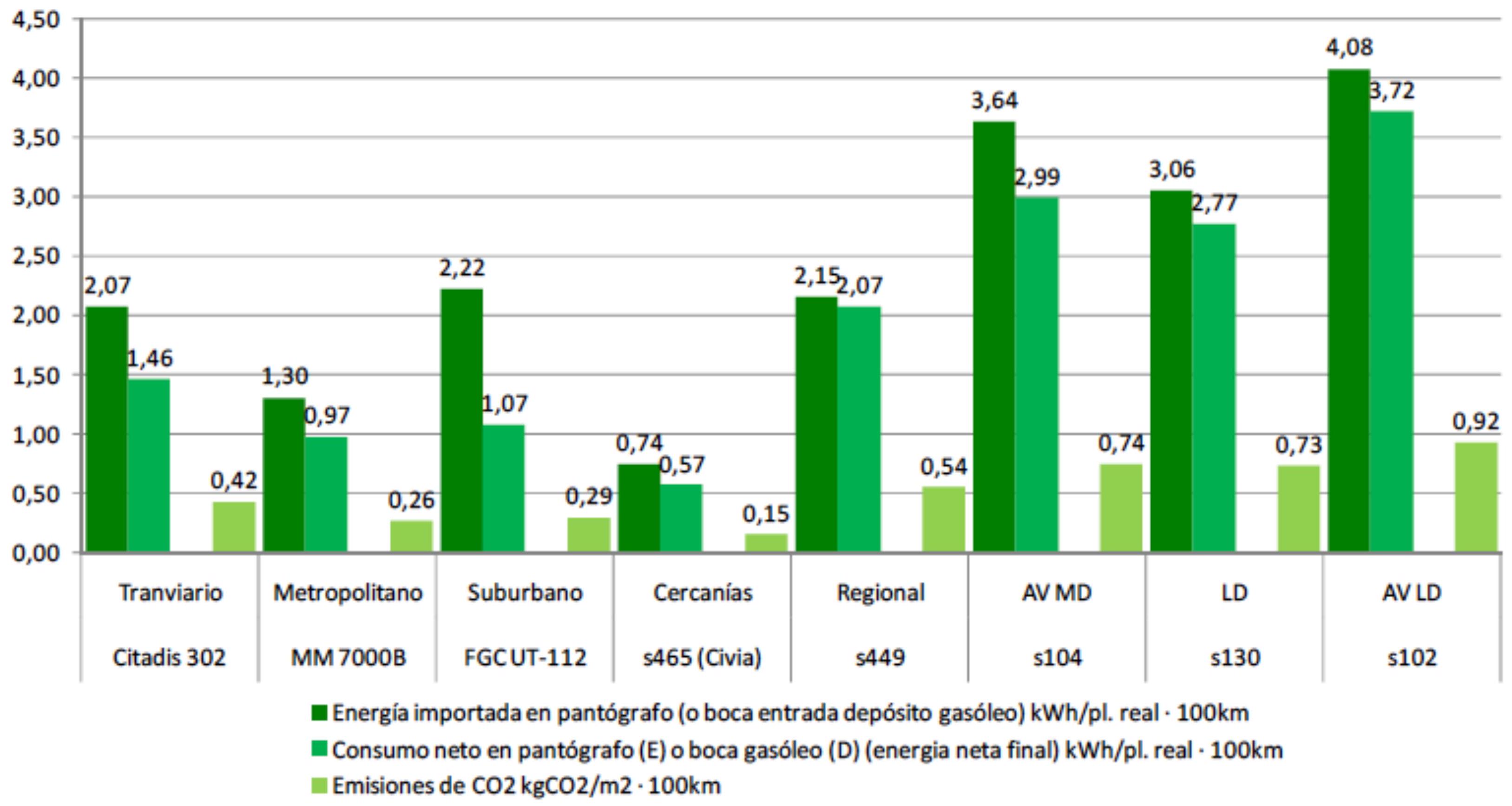
Consumption and Emissions per Real Seat per 100 km

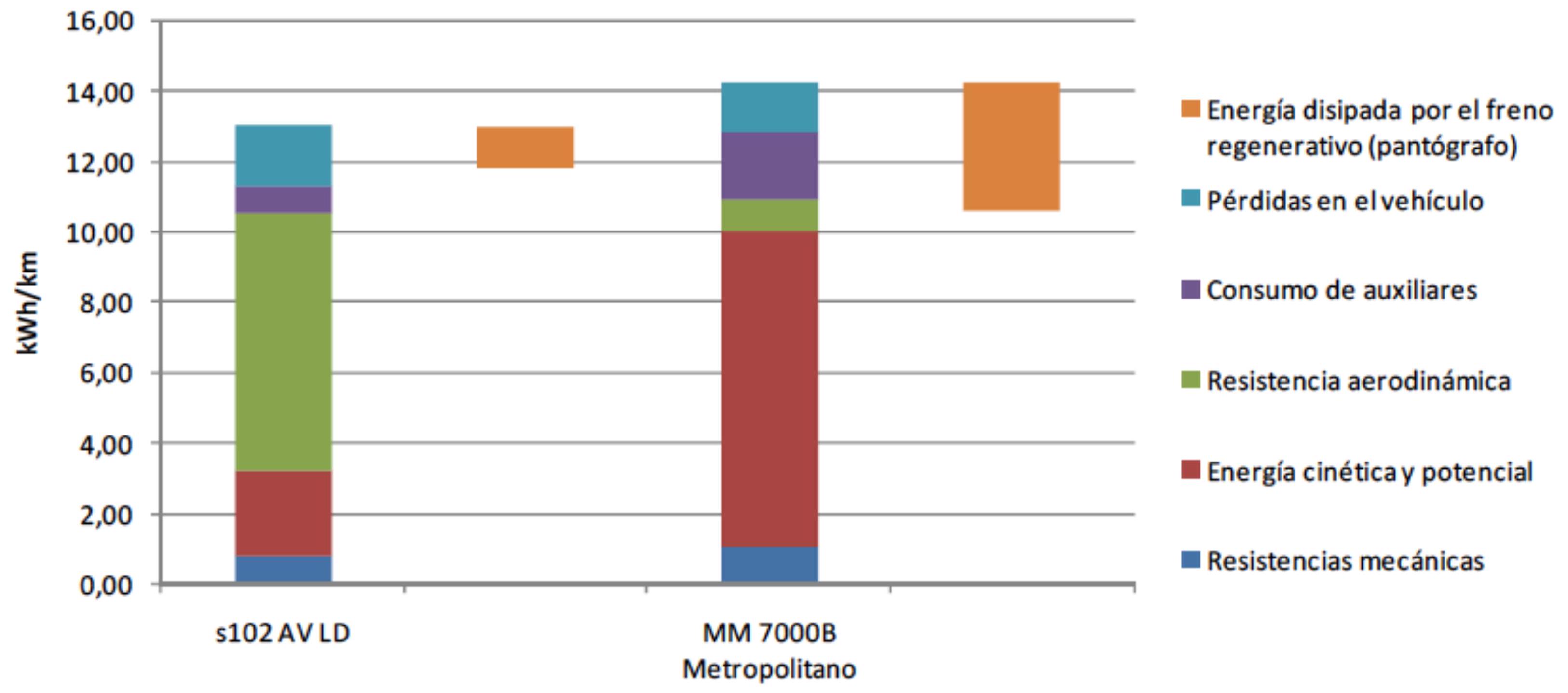
Breakdown of Imported Energy

Energy consumption and emissions analyses present significant variability according to railway vehicle type and service profile considered. This variability reflects different technical characteristics, operational speeds, passenger load profiles, and line configurations. To be able to establish meaningful comparisons between different railway services and evaluate their relative efficiency, it is indispensable to homogenize previously both nominal transport capacity and distance traveled by each vehicle.

A fundamental aspect in these analyses is that relative weight of each component of total consumption (mechanical resistance, aerodynamic resistance, energy dissipated in braking, technical and commercial auxiliaries) varies considerably function of train type and specific service. For example, high speed train on flat line presents consumption profile very different to conventional train on mountainous line, or freight train on mixed route. This difference of total consumption composition requires individualized analysis for each service and allows identifying specific opportunities for operational improvement and energy efficiency.

Chapter IV. Electrification

IV.1. Parts

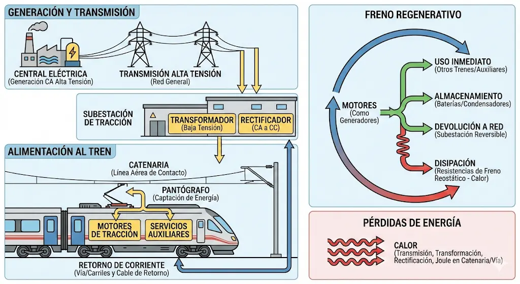
To adequately understand operation of railway electrification systems, it is fundamental to analyze their fundamental structure through traction circuit concept. This circuit represents physical and electrical path through which energy circulates from its generation to its utilization in locomotive.

The traction circuit is constituted by four essential components working in integrated manner:

• Energy Source: Substation acts as generating or transforming element of electrical energy.
• Supply Conductor: Contact line, commonly termed catenary, transmits current towards rolling stock.
• Consumer Element: Locomotive or motor units utilize supplied current to generate tractive effort.
• Return Conductor: Rail closes electrical circuit, allowing current to return towards substation.

A peculiar characteristic of this system lies in that, unlike conventional electrical circuits, railway traction circuit experiences continuous deformations in its geometry. Length and configuration of circuit vary constantly according to train position along line, since pantograph moves under catenary modifying continually distance between energy source and consumption point.

Regarding energy source, it is worth specifying that substation does not necessarily constitute primary origin of energy. In reality, it functions as intermediate element in integral electrical energy transport chain, connecting high voltage generating or transformer stations with track infrastructure. Substation performs critical transformation of current, adapting its voltage and intensity characteristics to specific requirements of railway line. In turn, substation receives supply from high voltage lines proceeding from energy generation centers.

Because coverage zone of a single substation possesses geographic limits determined by technical and economic considerations, it is necessary to distribute multiple substations along electrified lines. These substations are arranged in staggered manner, guaranteeing continuous and uniform coverage of railway infrastructure.

Contact Line

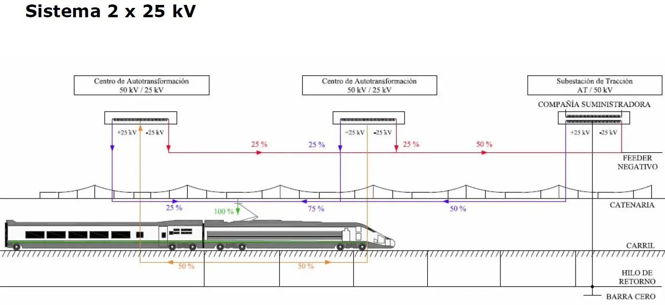
IV.2. Substations

Spatial distribution of substations along railway line constitutes critical design decision conditioned mainly by voltage drops occurring in conductors. The greater distance between substations, greater will be voltage losses in catenary and return rail, which can compromise efficient energy delivery to trains located far from nearest substation.

Voltage drop mitigation strategy depends fundamentally on current type used in electrification. In direct current systems, voltage drops are more severe due to linear relationship between conductor resistance and voltage loss. Consequently, to maintain acceptable performance parameters, it is necessary to reduce considerably distance between consecutive substations and employ conductors of significantly larger cross-section. In alternating current systems, on contrary, inductive effects allow greater distances without sacrificing efficiency, although this requires sophisticated transformers in substations.

Typical substation spacings in railway systems establish following guidelines:

• Direct Current: 20 Km
• Alternating Current: 50 Km

For urban transport systems like metros, where infrastructure is more compact and energy delivery requirements are higher, spacings reduce significantly to values oscillating between \(2-7 \mathrm{Km}\).

Following table presents standardized compilation of characteristic voltage levels of main railway electrification systems worldwide, establishing permitted minimum and maximum operational ranges:

Electrification System	Min. non-perm. voltage Umin.2(V)	Min. perm. voltage Umin. 1 (V)	Nominal Voltage Un (V)	Max. non-perm. voltage Umax1 (V)	Max. perm. voltage U max. 2 (V)
Direct current (mean values)		400	\(600{ }^{1)}\)	720	\(770{ }^{2)}\)
		500	750	900	\(950{ }^{3)}\)
		1000	1500	1800	1950
		2000	3000	3600	3900
Alternating current (RMS values)	11000	12000	15000	17250	\(18000{ }^{\text {4) }}\)
	17500	19000	25000	27500	29000

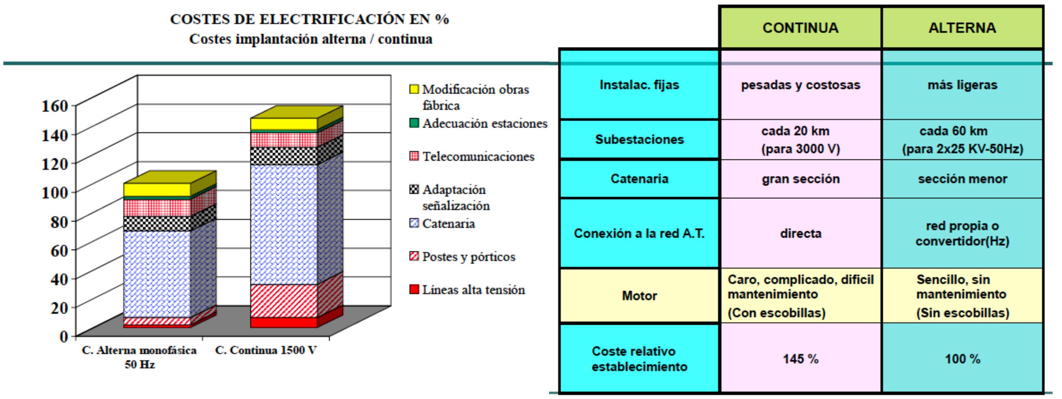
IV.3. Supply Systems

Specific configuration through which electrical energy is transmitted from substation to railway vehicle constitutes fundamental aspect of any electrification system. Term “catenary” is habitually used in railway field to designate aerial infrastructure acting as supply conductor, allowing electrical energy transfer to both locomotives and diverse rolling stock units.

In specialized technical literature, there exists alternative terminology that some engineers prefer to employ. Expression “Overhead Contact Line” (O.C.L.) provides more generic designation encompassing diverse types of aerial supply configurations, all characterized by presence of conductor or contact element suspended over track. This nomenclature integrates multiple system variants sharing similar fundamental principles:

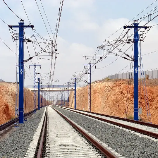
• Tramway line configurations, typically employed in urban transport systems
• Flexible catenaries, characterized by their elasticity and adaptability
• Rigid catenaries, providing greater structural stability

Parallel to these aerial supply systems, exist alternative technological solutions for energy distribution in railways which, although functioning under similar principles, cannot be classified strictly as catenaries. Among these alternatives, most significant is so-called “third rail”, representing fundamentally different solution for current delivery to rolling stock.

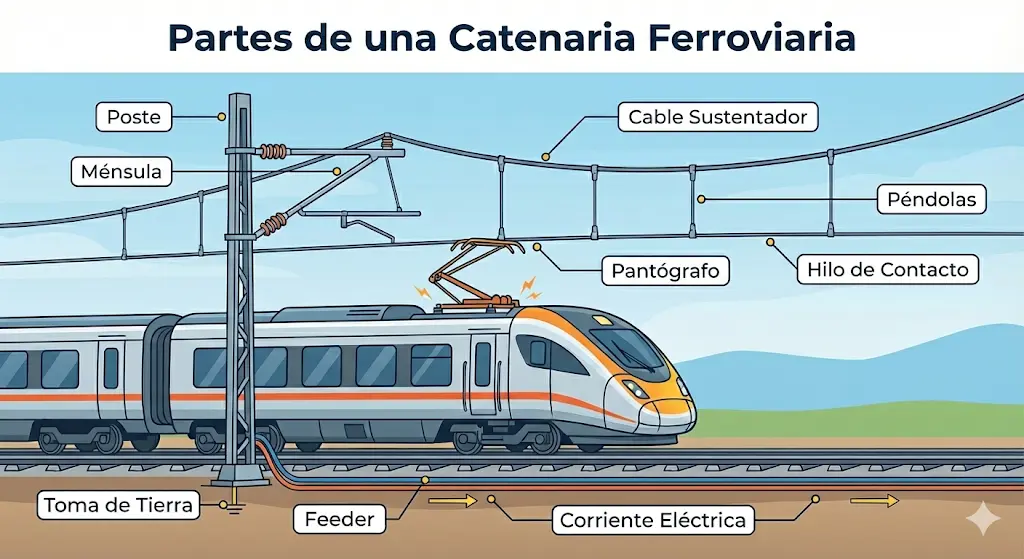
IV.3.1. Catenary

Catenary constitutes most widely used system in modern railway electrification installations, especially in long distance railways and rapid transit systems. This aerial supply system is based on principle of direct energy transmission through mechanical contact between pantograph mounted on vehicle roof and conductor or contact wire suspended over track.

Catenary experiences significant variations in its design and capacity according to voltage requirements of specific system. Constructive configurations adapt to different voltage levels employed, from low voltage DC systems to high voltage AC systems. Images presented below illustrate two representative examples of catenary configurations:

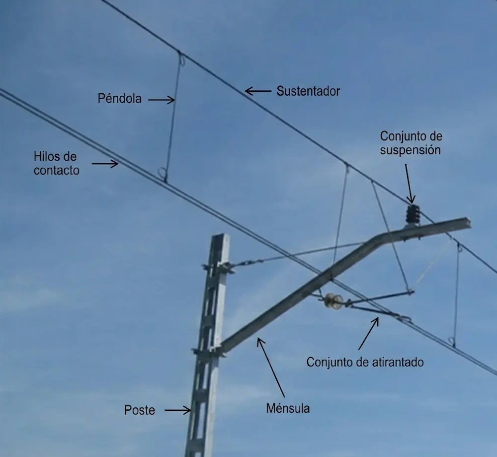Main elements of catenary

IV.3.2. Rigid Catenary

Rigid catenary represents technological variant of considerable importance differentiating fundamentally from conventional flexible catenary in its structural composition. Instead of employing flexible cable conductor, rigid catenary uses rigid metal rail as element transmitting electrical current. This rail possesses mechanical properties completely different to those of conventional cable, presenting significant bending stiffness.

From perspective of structural engineering, maintaining rigid rail in parallel position regarding railway track presents considerable technical challenges. Weight inherent to this structure is substantially greater than that of conventional cable, implying conventional tensioning or suspension methods by means of traction cables result insufficient. To guarantee structural stability and avoid excessive deformations, it is indispensable to increase significantly density of structural support points, reducing consequently distances between successive supports.

This engineering consideration generates very significant difference in utilized spacings. While rigid catenary requires spans (distances between consecutive supports) of approximately 10 to 12 meters, conventional flexible catenaries can reach spans in range of 50 to 60 meters, representing reduction of up to 80% in distance between supports. This structural limitation restricts drastically contexts in which rigid catenary results practically viable. Its implementation concentrates mainly in special environments like railway tunnels, structures with severe geometric limitations or layouts with very reduced clearances, where utilization of alternative systems becomes technically impossible or economically prohibitive.

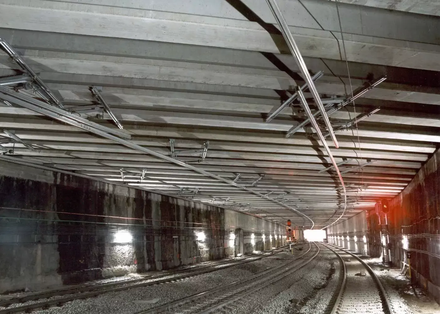
IV.3.3. Third Rail

In certain historical and particular contexts of railway engineering, completely different supply system known as “third rail” has been developed and implemented. This technological configuration represents fundamental alternative solution investing conventional paradigm of aerial supply. Instead of locating energy conductor suspended over track, third rail consists of installation of additional metallic supply rail, arranged longitudinally parallel to two main running rails and located at approximate height to ground level or slightly elevated. Energy transmission occurs through direct contact between elements termed shoes, mounted on lower part of railway vehicle, and supply rail surface.

Historical genesis of this system dates back to development of electrified railway transport in London Underground. When electrification of these urban railways began implementation, geometric restrictions of subterranean tunnels were extremely severe, leaving little clearance in upper zone to install conventional catenaries. This gauge limitation forced engineers to seek alternative solutions, resulting in innovative idea of locating supply system in lower part of tunnel, creating thus third rail concept.

Multiple constructive contact variations have been developed throughout years to optimize different aspects of this system’s performance. However, operational experience has demonstrated third rail presents significant limitations and risks advising widely against its use. Among main concerns are: firstly, creation of grave and potentially lethal electrocution risk for users and personnel who could accidentally fall on track, since supply conductor lies exposed at ground level; secondly, increased vulnerability to flooding phenomena and water accumulation, which can compromise electrical system integrity; and thirdly, fundamental functional incompatibility with aerial supply systems that could exist in other line segments, complicating operational integration. For these reasons, use of third rail is currently restricted to those very specific situations where implementation of superior supply systems results technically impossible or economically unfeasible.

IV.3.4. Pantograph

Pantograph constitutes critical mechanical and electrical component performing capture and reception of current from supply line towards railway vehicle. This device is firmly secured to upper structure of locomotive or motor car, extending vertically upwards in direction to catenary. Fundamental engineering aspect in pantograph design lies in its electrical insulation regarding rest of vehicle metallic structure, achieved through incorporation of high specification porcelain insulators preventing uncontrolled current flow towards train chassis.

From perspective of contact dynamics, interaction between pantograph and catenary contact wire generates mechanical forces of considerable magnitude. Pantograph exerts normal pressure on catenary in range of \(300-400 \mathrm{~N}\), necessary to guarantee reliable low resistance electrical contact, but simultaneously generating wear effects on both contacting surfaces.

To mitigate detrimental effects of excessive localized wear on contact elements known as strips (pantograph contact surfaces), load lateral distribution strategy has been adopted through catenary implantation according to zig-zag pattern perpendicular to track longitudinal axis. This alternating configuration produces that pantograph, during its movement along line, performs sequential contact with different lateral positions of contact wire, distributing thus wear over more extensive surface and prolonging significantly useful life of both components.

Review Questions

What is the fundamental equation of longitudinal movement of a train?

It is \(E-R=\frac{P}{g} \cdot \gamma\), where E is tractive effort, R resistances, P weight and \(\gamma\) acceleration.

On what variables does the adhesion limit mainly depend to prevent wheel slip?

It depends on adhesive weight (\(P_{adh}\)) and coefficient of adhesion (\(\phi\)), according to relationship \(F \leq \phi \cdot P_{adh}\).

What are the three main components of resistance to motion of a train?

Mechanical resistances (rolling and frictions), resistance by air intake and aerodynamic resistances (pressure and friction).

What four fundamental elements constitute electrical traction circuit?

Substation (source), catenary (supply conductor), locomotive (consumer) and rail (return conductor).

Why does rigid catenary require much smaller distance between supports (10-12m) than flexible?

Because rigid rail has much greater weight than flexible cable, requiring more support points to avoid structural deformations.

Bibliography

• Díaz de Villegas, J.M. (2003) Ferrocarriles. Course Notes. E.T.S. Ing. Caminos, Canales y Puertos Santander.
• García Álvarez, A. (2022) Manual de ferrocarriles. El sistema ferroviario español. Ed. Garceta.
• M. Melis and F. Gonzalez, Ferrocarriles metropolitanos. Tranvías, metros ligeros y metros convencionales. \(3^{\mathrm{rd}} \mathrm{Ed}\)., Colegio de Ingenieros de Caminos, Canales y Puertos., 2008.
• Proyecto ElecRail. [Online]. Available: http://www.investigacionffe.es/elecrail_publicaciones.asp.
• Gonzalez Franco, I. (2021) Apuntes de Dinámica del ferrocarril: Esfuerzos de tracción y resistencias al avance. Modelos de Cálculo de Energía Consumida. Master in Railway Engineering UC-Mafex.
• https://www.tool.es/web/SimulaFFCC.html