Fundamentals of Railway Mechanics: Analysis of Vertical and Transverse Behavior of the Infrastructure
Table of contents
Chapter I. Track Elasticity
In granular materials such as ballast, as well as in the natural ground layers that support it, and generally in any medium formed by discrete particles, when a load is applied for the first time, a deformation of an irreversible nature is generated, known as plastic deformation. However, when these stresses are repeated consecutively for a considerably high number of cycles, the mechanical behavior of the material transitions towards a state of true elasticity, characterized by responses similar to those experienced by monolithic and homogeneous solids.
To adequately quantify and characterize this elastic property present in the railway track structure, various mathematical parameters and behavioral models are used to capture the most relevant aspects of this response.
I.1. TRACK MODULUS K
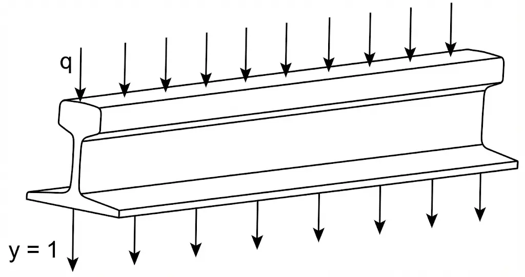
Considering that \(\boldsymbol{q}(\boldsymbol{t} / \boldsymbol{m})\) represents a uniformly distributed load along the length of a rail, and identifying \(y\) as the vertical settlement or subsidence produced in the rail as a result of the application of said load.
From a physical meaning perspective: this parameter represents the load magnitude that, when acting uniformly and continuously on the rail, generates a vertical displacement of unit magnitude in it.
This modulus is particularly used in American and Canadian railway engineering contexts. When the unit of settlement considered is 1 centimeter, the track modulus K is typically within the range of 8 to 22 tons per linear meter.
I.2. SLEEPER REACTION COEFFICIENT R
This parameter was initially proposed by the researcher and professor Timoshenko in 1915 as part of his fundamental work in structural mechanics. In this context, \(\boldsymbol{R}\) is defined as the vertical reaction emerging at the sleeper, being evaluated specifically for each of the support rails, while \(\boldsymbol{y}\) represents the settlement or vertical displacement produced at that evaluation point (measured in tons per millimeter).
\[r=\frac{R}{y}\]An equivalence relationship can be established between the track modulus K and the coefficient r if the distance d corresponding to the spacing between two successive sleepers is introduced:
\[r=\frac{R}{y}=R \cdot \frac{K}{r}=d \cdot r \cdot \frac{K}{r}=K \cdot d\]From which the following relationships are derived: \(K=\frac{r}{y}\) and \(R=r \cdot d\)
It should be noted that this relationship constitutes an approximation to reality, since its formulation has omitted the effect of mutual influence exerted by adjacent and neighboring sleepers on each other.
I.3. BALLAST COEFFICIENT C
\[C=\frac{r}{S}\]This coefficient was proposed by Winkler in 1867 and represents the relationship between the elastic reaction and the contact area. In this expression, \(\boldsymbol{S}\) corresponds to the support surface presented by the sleeper at its interface with the ballast. If we represent by P (in k/cm²) the average pressure transmitted over the support zone \(S\) of the sleeper:
\[C=\frac{r}{S}=\frac{R}{y \cdot S}=\frac{P}{y}\]From this formulation, the ballast coefficient can be physically interpreted as the unit pressure that, when applied to the ballast material, produces a depression or settlement of exactly 1 centimeter in it. To illustrate this concept through a practical example: consider a sleeper supported on ballast that transmits a pressure of \(\mathbf{2}\) K/cm² and generates a settlement of \(\mathbf{0.05}\) cm; in this case, the resulting ballast coefficient would be:
\[C=\frac{P}{y}=\frac{2 \mathrm{k} / \mathrm{cm}^{2}}{0.05 \mathrm{~cm}}=40 \mathrm{k} / \mathrm{cm}^{3}\]This parameter changes notably with the process of tamping (packing) the ballast. According to practice and experience in railway infrastructure design, the ballast coefficient should typically be maintained within the interval of \(5-10\) K/cm³.
I.4. ELASTICITY COEFFICIENT
The railway track infrastructure is composed of an integrated system of multiple layers and materials, each of which presents differentiated individual elastic characteristics (support subgrade, ballast layer, sleepers, rails, fastenings, etc.). For each of these constituent components, it is possible to assign a specific elasticity coefficient denoted as \(\boldsymbol{r}_{\boldsymbol{n}}\), which is established by definition as follows:
\[r_{n}=\frac{R}{y_{n}}\]Considering that y represents the total accumulated vertical settlement or deformation resulting from the superposition of all individual deformations of each component:
\[y=\sum_{n} y_{n}=\sum_{n} \frac{R}{r_{n}}=R \cdot \sum_{n} \frac{1}{r_{n}}=\frac{R}{r}\]In accordance with various studies and experimental records obtained in railway engineering projects, the typical elasticity coefficients for each structural element of the track are:
| Component | Stiffness (t/mm) | Observations |
|---|---|---|
| Rail web | \(5000 - 10000\) | The component with the highest stiffness. |
| Concrete sleeper | \(1200 - 1500\) | Significantly stiffer than wood. |
| Wooden sleeper | \(50 - 80\) | Higher elasticity than concrete. |
| Tamped ballast | \(10 - 30\) | Increases with thickness and decreases over time. |
| Rocky subgrade | \(2 - 8\) | - |
| Clay subgrade | \(1.5 - 2\) | - |
| Swampy subgrade | \(0.5 - 1.5\) | The component with the lowest stiffness. |
From a perspective of the global behavior of the track structure, it is precisely the ballast and the support subgrade that are the elements exerting the most determining influence on the elastic characteristics of the complete railway infrastructure set.
\[y=\sum_{n} y_{n}=\sum_{n} \frac{R}{r_{n}}=R \cdot \sum_{n} \frac{1}{r_{n}}=\frac{R}{r}\]The consolidated reaction coefficient representing the entire structure can fluctuate within a fairly wide range comprised between \(\mathbf{1.5 - 1 0}\) t/mm, depend essentially on the characteristics and properties of the ballast material used and the geological nature and composition of the underlying subgrade. The value most commonly found in conventional railway engineering projects is approximately \(\mathbf{3}\) t/mm.
In special contexts, such as structures built on civil works, bridges, or other artworks, notably higher values are obtained within the range \(12-15\) t/mm, evidencing a significant difference in stiffness properties.
It should be highlighted that the subgrade is the component presenting the lowest elastic coefficient in the load transmission chain, which is why the specific pressure exerted at the level of this subgrade becomes the parameter that fundamentally conditions the total track settlement. This pressure on the subgrade results to be lower the greater the thickness of the ballast layer interposed between it and the upper structure.
I.5. Load Classification
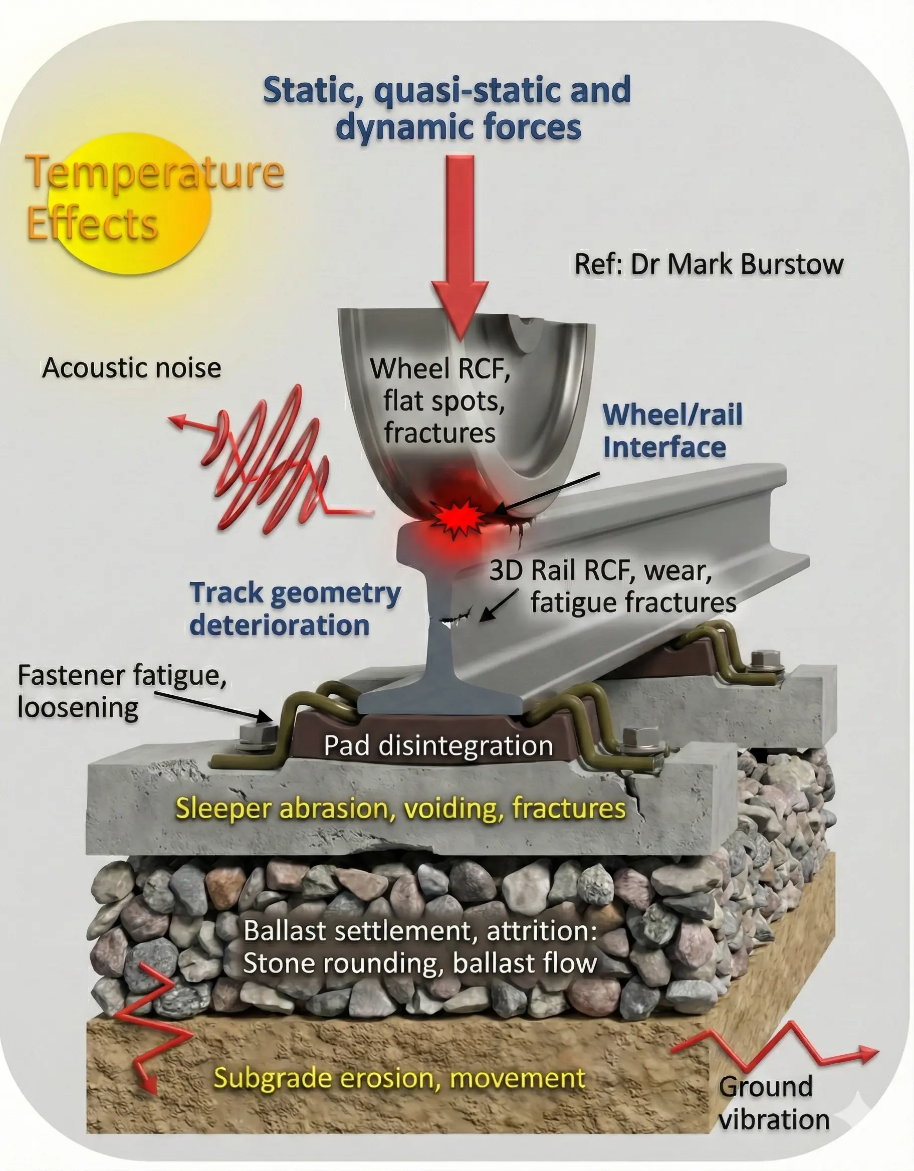
Railway infrastructure constitutes a system subjected to a heterogeneous set of mechanical stresses of diverse nature. These loads can be classified according to their direction and sense of application into the following main categories:
Vertical Loads: These are applied on the running surface of the rail and are transmitted towards the lower ground layers through the chain of track structural components, including sleepers, ballast, and subgrade.
Transverse Loads: Initially transferred from the wheel-rail contact towards the rails, which can be effected solely through the running surface (when there is no contact of the wheel flanges with the rail) or involving simultaneously the running surface and mainly the wheel flanges (when lateral movement causes flange contact). Subsequently, these loads propagate towards the lower structures through intermediate components such as fastenings, base plates, and sleepers.
Longitudinal Loads: Applied tangentially on the rail running surface and transmitted to the lower layers in a manner analogous to transverse loads, using the same force distribution route.
Excluding extraordinary events such as seismic phenomena, it is important to emphasize that all dynamic forces and stresses acting on the railway track are generated and transmitted by the rolling stock circulating on the infrastructure (traffic-derived loads).
According to the temporal nature of their application, the loads acting on the track are further subdivided into the following categories:
Static loads: Those resulting from the inherent dead weight of the rolling stock and its components. These loads are exerted permanently and continuously on the track, regardless of whether the rolling stock is stationary or in motion.
Semi-static or quasi-static loads: These stresses are transmitted to the rolling stock and consequently to the track during specific and determined time intervals. Once the cause originating them ceases, they disappear immediately. Representative examples include residual centrifugal force not completely compensated and forces generated by crosswinds.
Dynamic loads: These originate and are generated as a consequence of multiple concurrent factors:
- Irregularities and defects present in the track geometry and alignment, as well as the variability or heterogeneity in the vertical stiffness of the structure.
- Discontinuities and abrupt changes in the running surface geometry (such as rail joints, switch zones, crossings, etc.).
- Progressive wear of the running surface on both rails and rolling stock wheel flanges.
- Characteristics of the vehicle suspension system and asymmetries inherent to the design and construction of the rolling stock.
I.6. Vertical Loads
Complementing the three categories described above, it is equally relevant to consider and analyze specifically an additional category of vertical stresses that can be termed as “characteristic loads” defining the track behavior. This subcategory encompasses the following components:
- The axle load Q
- The equivalent daily fictitious traffic \(T_{f}\)
- The vertical design wheel load \(Q_{d}\)
A distinctive and fundamental characteristic of all these characteristic loads, which can present both static and dynamic nature, is that they exert a determining influence on the dimensioning and design processes of the railway infrastructure, as well as on the preventive and corrective maintenance strategies and policies that must be implemented throughout the useful life of the track.
I.6.1. Quasi-Static Vertical Loads
Axle load
The term “axle load” is used to designate the magnitude of vertical load of static nature Q transmitted and transferred by each component axle of a railway vehicle, and in a broader sense of a complete train, towards the rails through its contact wheels.
Under the fundamental hypothesis that the load is distributed symmetrically across the different constituent parts of the vehicle, the magnitude of the axle load is mathematically expressed as the quotient between the total weight of the vehicular unit and the total number of axles composing the train.
In the particular case of a vehicle equipped with conventional bogies possessing two axles each, the axle load is calculated applying the following mathematical expression:
\[Q=\left(\frac{\bar{M}}{4}+\frac{M^{\prime}}{2}+m\right) \cdot g\]where the terms are defined as: Q: Magnitude of the load transferred by each axle. \(\bar{M}\) : Mass of the vehicle body structure. \(\mathrm{M}^{\prime}\) : Mass of each of the bogies. m: Mass of a complete railway wheelset assembly, including the axle, wheels, and all associated components such as axle boxes. g: Acceleration caused by terrestrial gravity.
The International Union of Railways (UIC) has established a systematic classification of railway tracks based on the maximum load capacity allowed per axle, dividing them into four service categories or levels: A, B, C, and D:
| Track category | Axle load \((t)\) |
|---|---|
| A | 16 |
| B | 18 |
| C | 20 |
| D | 22.5 |
Source: Adapted from UIC. 1989, Fiche 714R, Classification des voies des lignes au point de vue de la maintenance de la voie.
It is important to recognize that the maximum allowed axle load varies considerably from one railway country to another, and even within the same country, significant variations may exist from one railway line to another.
A practical aspect of considerable relevance is that increasing the track gauge (broad gauge) allows and facilitates a significant increase in the load transferred by each axle. Additionally, axle loads exceeding \(Q>16-17\) t are generally considered prohibitive or incompatible with the development of very high circulation speeds (exceeding \(V \geq 250\) km/h) for safety and comfort reasons.
Wheel load
The term “wheel load” refers to the magnitude of the vertical load of static nature \(\mathbf{Q}_{\mathbf{o}}\) transmitted by each individual vehicle wheel towards its corresponding contact point on the rail.
Considering symmetrically distributed load conditions in the vehicular unit, the wheel load is obtained through the following mathematical relationship:
\[Q_{o}=\frac{Q}{2}\]In real practical contexts, particularly when the vehicle circulates on curved trajectories, it is observed that the loads transmitted by the two wheels of the same axle are not identical to each other, presenting an unequal distribution.
The individual load of each wheel, with special emphasis on the differential weight distribution between both wheels, maintains a direct and significant relationship with critical derailment phenomena and possible overturning of railway vehicles.
Daily Fictitious Traffic
The determination of the quantity and characteristics of traffic circulating on a track is typically performed by introducing the concept of daily fictitious traffic \(\boldsymbol{T}_{\boldsymbol{f}}\) (expressed in tons). This parameter constitutes one of the most important so-called “characteristic loads”. By evaluating the total value of this daily fictitious traffic, it is possible to classify railway tracks into different categories, thus allowing the normalization and standardization of structural dimensioning criteria and infrastructure preventive maintenance programs.
To carry out the systematic calculation of \(\boldsymbol{T}_{\boldsymbol{f}}\), the international organization UIC has proposed and recommended two different mathematical formulations that can be used depending on the specific characteristics of each infrastructure:
\[T_{f}=T_{p} \cdot \frac{V_{\text {max }}}{100}+T_{g} \cdot \frac{Q_{D_{o}}}{18 \cdot D_{o}}\]where:
| Track category | Total daily traffic load \((t)\) |
|---|---|
| I | \(T_{\mathrm{f}}>40,000\) |
| II | \(40,000 \geq T_{\mathrm{f}}>20,000\) |
| III | \(20,000 \geq T_{\mathrm{f}}>10,000\) |
| IV | \(10,000 \geq T_{\mathrm{f}}\) |
\(T_{f}\) : Daily fictitious traffic (in t). \(T_{p}\) : Passenger train traffic (in t). \(T_{g}\) : Freight train traffic (in t). \(V_{\text {max }}\) : Maximum circulation speed (in km/h). \(D_{0}\) : Minimum wheel diameter of trains circulating on the line (in m). \(Q_{D o}\) : Maximum load per passing axle (wheels of diameter Do) (in t).
| Track category | Total daily traffic load ( \(T_{p}\) ) |
|---|---|
| UIC I | \(130,000 \mathrm{t}<\mathrm{T}_{6}\) |
| UIC 2 | \(80,000 \mathrm{t}<\mathrm{T}_{\mathrm{r}} \leq 130,000 \mathrm{t}\) |
| UIC 3 | \(40,000 \mathrm{t}<\mathrm{T}_{\mathrm{f}} \leq 80,000 \mathrm{t}\) |
| UIC 4 | \(20,000 \mathrm{t}<\mathrm{T}_{\mathrm{f}} \leq 40,000 \mathrm{t}\) |
| UIC 5 | \(5,000 \mathrm{t}<\mathrm{T}_{1} \leq 20,000 \mathrm{t}\) |
| UIC 6 | \(\mathrm{T}_{4} \leq 5,000 \mathrm{t}\) |
Source: Adapted from UIC. 1989, Fiche 714R, Classification des voies des lignes au point de vue de la maintenance de la voie.
\[T_{f}=S_{v} \cdot\left(T_{V}+K_{t}+T_{t v}\right)+S_{m} \cdot\left(K_{m} \cdot T_{m}+K_{t} \cdot T_{t m}\right)\]where: \(T_{f}\) : Daily fictitious traffic (in t). Tv: Average daily traffic of hauled passenger coaches (in t). \(T_{m}\) : Average daily traffic of freight wagons (in t). \(T_{t v}\) : Average daily traffic of passenger locomotives (in t). Ttm: Average daily traffic of freight locomotives (in t). \(K_{m}\) : Coefficient with values ranging between 1.15 (standard value) and 1.45 (when > \(50 \%\) of traffic is with vehicles with axle load \(\mathrm{Q}=22.5 \mathrm{t}\) or when \(75 \%\) of traffic is with vehicles of axle load \(\mathrm{Q} \geq 20 \mathrm{t}\)). \(K_{t}\) : Coefficient depending on the rolling conditions of locomotive axles on the track. Usually equal to 1.40. \(S_{v}, S_{m}\) : Coefficients whose values depend on the speed of passenger trains (with the highest speed) and freight trains (with the lowest speed), respectively, circulating on the track.
Vertical wheel load due to crosswinds
Atmospheric stresses exert significant influences on the dynamic behavior of railway vehicles. The vertical load induced by crosswinds \(\mathbf{Q}_{\boldsymbol{w}}\) represents the redistribution of vertical loads between the wheels of the same axle, resulting from the action of transverse wind forces on the vehicle body. This load is quantified by the mathematical expression presented in the following equation (Esveld, 2001):
\(\pm Q_{w}=H_{w} \cdot \frac{q_{o}}{a}\)
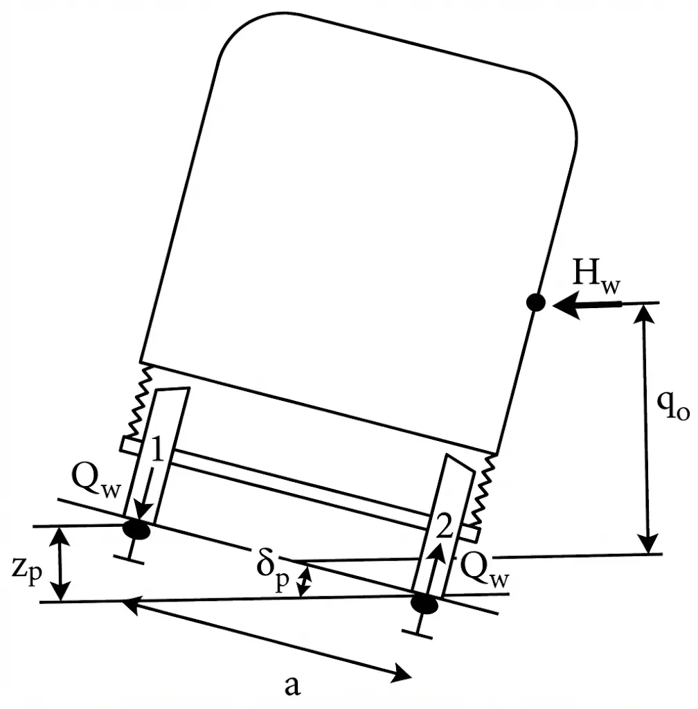 In this expression, the parameters are defined as follows:
\(H_{w}\) : Transverse wind force applied at the geometric center of the body lateral surface.
\(q_{o}\) : Vertical distance between the geometric center of the body lateral surface and the rail running surface.
a: Distance between the vertical symmetry axis of the two rails.
In this expression, the parameters are defined as follows:
\(H_{w}\) : Transverse wind force applied at the geometric center of the body lateral surface.
\(q_{o}\) : Vertical distance between the geometric center of the body lateral surface and the rail running surface.
a: Distance between the vertical symmetry axis of the two rails.
The load distribution mechanism works such that when the horizontal wind force \(H_{w}\) is directed from wheel 2 towards wheel 1, the load supported by wheel 1 increases by the amount \(Q_{w}\), while simultaneously the load of wheel 2 experiences a decrease of identical magnitude. This characteristic reveals the redistributive character of transverse stresses.
From a temporal perspective, the load originated by crosswinds manifests solely during vehicle movement, both on straight track segments and on curved sections, persisting as long as wind conditions remain. Once such climatic conditions cease, the stress disappears, returning the system to its initial static load state.
Vertical wheel load due to unbalanced centrifugal force
In the context of movement in curves, the incomplete compensation of centrifugal acceleration through track stiffness (cant) generates a residual force transmitted to the track structure. The vertical load induced by this unbalanced centrifugal force \(Q_{s c}\) is expressed mathematically as indicated in the following equation, establishing the relationship between the residual force and vertical load redistribution (see attached figure):
\(\pm Q_{s c}=\frac{F_{s c} \cdot h_{k B}}{a}=\frac{Q \cdot I \cdot h_{k B}}{a^{2}}\)
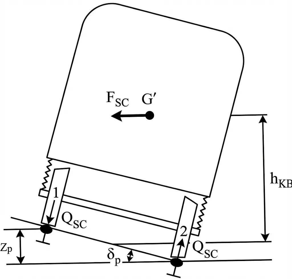 The terms integrating this formulation are defined as follows:
\(F_{s c}\) : Unbalanced centrifugal force.
I: Cant deficiency.
\(h_{\text {кв }}\) : Distance between the vehicle center of gravity \(\mathrm{G}^{\prime}\) and the rail running surface.
\(z_{p}\) : Track cant.
\(\delta_{p}\) : Cant angle.
The terms integrating this formulation are defined as follows:
\(F_{s c}\) : Unbalanced centrifugal force.
I: Cant deficiency.
\(h_{\text {кв }}\) : Distance between the vehicle center of gravity \(\mathrm{G}^{\prime}\) and the rail running surface.
\(z_{p}\) : Track cant.
\(\delta_{p}\) : Cant angle.
The magnitude of the quasi-static load derived from centrifugal deficiency presents particular characteristics: it activates exclusively during vehicle displacement in curved infrastructure sections, and typically adopts values within the interval of \(\mathbf{1 0 - 2 5 \%}\) of the nominal static wheel load, depending on the curve’s geometric and dynamic parameters. Regarding transverse distribution, the wheel circulating on the outer rail experiences a load increase of magnitude \(Q_{s c}\), while the inner wheel simultaneously records a proportional decrease of identical amount, thus establishing a redistributive equilibrium in the axle load system.
I.6.2. Dynamic Vertical Loads
The interaction between rolling stock and railway infrastructure generates complex dynamic phenomena introducing fluctuating stresses superimposed on the previously analyzed static and quasi-static loads. These dynamic loads constitute the manifestation of vibration and impact mechanisms deriving from both the vehicle’s constructive characteristics and geometric irregularities present in the track.
The total dynamic vertical wheel load \(\left(\mathbf{Q}_{\text {dyn }}\right)\) is the sum of:
- vehicle suspended masses ( \(\mathbf{Q}_{\text {dyn1 }}\) ): Vehicle body
- vehicle semi-suspended masses ( \(Q_{\text {dyn2). }}\) Bogies
- vehicle unsuspended masses ( \(Q_{\text {dyn3). Axles}}\)
- masses due to oscillations of elastic parts of the rail-sleeper fastening system ( \(Q_{\text {dyn4 }}\) ).
The nature of dynamic forces exerted on the track during interaction with rolling stock is predominantly random, non-deterministic. This characteristic grounds the need for a probabilistic and statistical treatment in their analysis.
By applying the structural response linearity hypothesis, the study of dynamic phenomena can be subdivided into different frequency ranges, according to the specific oscillation mechanism in question, the vibration originating cause, and the participating structural or vehicle component in the oscillatory movement.
Consequently, the total vertical dynamic wheel load \(\boldsymbol{Q}_{\boldsymbol{d} \boldsymbol{y}}\) is obtained by the weighted sum of all identified dynamic force categories:
\[Q_{d y n j}=Q_{d y n 1 j}+Q_{d y n 2 j}+Q_{d y n 3 j}+Q_{d y n 4 j}\]In this expression: \(\mathrm{j}=1,2\) : Subscript indicating each of the two wheels composing a wheelset.
The historical evolution of railway systems has demonstrated that increasingly higher speeds, combined with progressive increases in vehicle weight and greater stiffness of infrastructure components, generate a substantial increase in the magnitude of dynamic effects, resulting in a significant increase in stresses transmitted to the track superstructure, the seating subgrade, and vehicle components.
From a methodological perspective, the precise calculation of dynamic forces continues to be a problem of considerable analytical complexity, frequently intractable by purely analytical methods. In professional practice, most analyses are limited to simplified quasi-static approximations. However, the predominant approach in modern engineering consists of adopting empirical methodologies grounded in experimental measurement data (Giannakos, 2014, 2016).
The magnitude of the additional dynamic load can reach values as high as \(50 \%\) of the nominal static wheel load (Alias, 1977). According to specialized technical literature (Profillidis, 1995; Zicha, 1989), in the speed range up to 200 \(\mathrm{km} / \mathrm{h}\), the dynamic impact coefficient typically fluctuates between 1.35 and 1.6. For this reason, for speeds not exceeding 200 \(\mathrm{~km} / \mathrm{h}\), the adoption of a dynamic impact coefficient of 1.5 in design is recommended. For speeds exceeding \(200 \mathrm{~km} / \mathrm{h}\), it is prudent to perform detailed analytical studies grounded in specific experimental data of the infrastructure under study.
I.6.3. Total Vertical Wheel Load
The integral quantification of the vertical stress transmitted by rolling stock towards the track structure requires the joint consideration of all load components identified in preceding sections. The total vertical wheel load \(Q_{t}\) represents the stress envelope, expressed as the algebraic composition of nominal static vertical loads, quasi-static additions derived from environmental and curvature effects, and random dynamic fluctuations:
\[Q_{t j}=Q_{o j} \pm Q_{w j} \pm Q_{s c j} \pm Q_{d y n j}\]This integral expression provides the reference framework for evaluating the track structural response to the passage of railway traffic.
I.6.4. Design Vertical Wheel Load
The railway infrastructure design methodology requires the establishment of a representative stress parameter encapsulating the statistical probability of not being exceeded during the track’s useful life. This parameter is termed “design vertical wheel load” \(\mathbf{Q}_{\boldsymbol{d}}\), and represents the characteristic value of vertical stress which, from a probabilistic perspective, is associated with the maximum theoretical probability of not being exceeded under real operating conditions throughout the complete infrastructure lifecycle.
The formulation of the design vertical load incorporates a rigorous statistical treatment recognizing the random nature of dynamic phenomena. The design load \(\boldsymbol{Q}_{\boldsymbol{d}}\) is calculated as the integrated sum of the nominal static component, the quasi-static contribution (derived from environmental and geometric conditions), and a term representing the statistical dispersion of dynamic forces, weighted by a probability factor. This statistical weighting ensures a probabilistic safety margin against load exceedances under operational conditions. The mathematical formulation expressing this concept comes from specialized literature (Esveld, 2001; Giannakos, 2002) and is presented below:
\[Q_{d j}=Q_{o j}+Q_{H j}+n_{p} \cdot \sqrt{\sigma\left(Q_{d y n 3 i}\right)^{2}+\sigma\left(Q_{d y n 1 i}+Q_{d y n 2 i}\right)^{2}}\]The terms integrating this equation are defined as specified below: \(\mathrm{Q}_{\mathrm{d}}\) : Vertical design wheel load. Qo: Static component of vertical wheel load. \(Q_{H}\) : Quasi-static component of vertical wheel load. \(\sigma\left(Q_{\mathrm{dyn}}\right)\) : Standard deviation of vertical dynamic forces associated with vehicle unsuspended masses. \(\sigma\) ( \(Q_{\text {dyn1 }}, Q_{\text {dyn2) }}\) : Standard deviation of vertical dynamic forces corresponding to suspended and semi-suspended vehicle masses. \(\mathrm{n}_{\mathrm{p}}\) : Multiplier coefficient amplifying the root mean square value of dynamic standard deviations, ensuring coverage of statistical non-exceedance probability during the infrastructure’s useful life. This coefficient typically adopts a value of 5.00 (Demiridis and Pyrgidis, 2010). \(\mathrm{j}=1,2\) : Subscript index indicating each of the two wheels of the same wheelset of an axle.
I.7. Transverse Loads
Transverse stresses constitute a critical aspect for evaluating the operational safety of the railway system. These forces are directly linked to both the kinetic safety of railway circulation and the dynamic comfort perceived by passengers, being capable of triggering the critical derailment phenomenon.
Transverse forces can be classified into two fundamental categories according to their origin mechanism:
I.7.1. Forces caused by wheel-rail interaction
This category comprises a set of forces derived from the interaction dynamics between vehicle rolling elements and the infrastructure. It includes: gravitational or restoring forces derived from wheel conicity, guiding forces emerging upon contact of wheel flanges with rails, friction forces both transverse and longitudinal resulting from relative sliding at the contact point, and dynamic forces associated with vehicle oscillations. Friction forces are additionally subdivided into transverse and longitudinal components.
A second category of transverse forces is originated by effects exogenous to conventional circulation dynamics. This category, termed “forces due to other causes”, encompasses uncompensated centrifugal force derived from movement in curves with cant deficiency, as well as atmospheric wind transverse force.
I.7.2. Gravitational Forces
At the wheel-rail contact point, the global normal reaction \(\boldsymbol{R}_{\mathbf{o}}\) can be decomposed into two orthogonal components: a vertical component \(\boldsymbol{Q}_{\mathbf{o}}\) (wheel load) and a transverse component \(\boldsymbol{S}_{\boldsymbol{p o}}\) (see reference figure). The transverse component \(\mathrm{S}_{\mathrm{po}}\), termed “gravitational force”, “restoring force” or “gravitational stiffness”, constitutes a re-centering mechanism acting to maintain the wheelset in its equilibrium position on the track. This force is caused exclusively by the conical geometry of the wheel tread, being transmitted through the axle towards the rail running surface.
It is considered a dynamic nature force and mathematically expressed according to:
\(S_{p o}=Q_{o} \cdot \tan \gamma_{o}\)
in which:
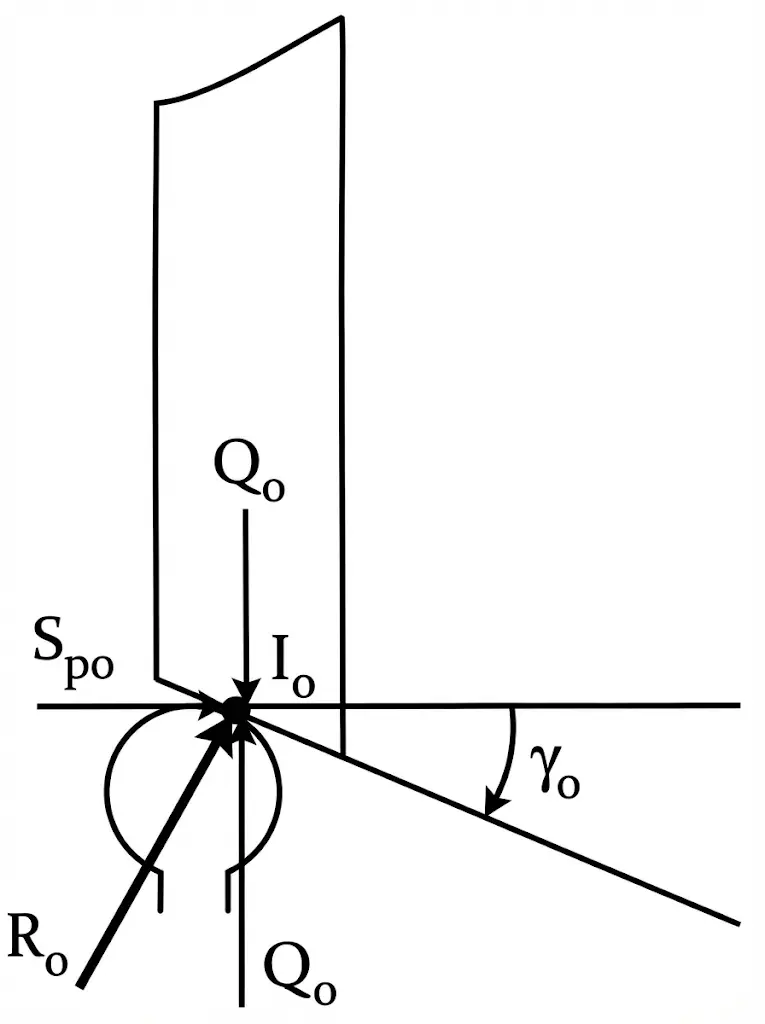
Qo: Static wheel load. \(\gamma_{o}\): Surface inclination angle with respect to the horizontal plane in the wheel’s central equilibrium position.
In the case of a conventional wheelset, each of the two wheels generates its own gravitational force ( \(\boldsymbol{S}_{\boldsymbol{p} j,} \mathrm{j}=1,2\) ), as schematically illustrated in the attached figure.
When a transverse displacement of the wheelset occurs, symbolized by “y”, the asymmetric distribution of wheel-rail contact originates variations in individual gravitational forces. The mathematical expressions describing this behavior are:
\(S_{p 1}=Q_{1} \cdot \tan \gamma_{1}=Q_{1} \cdot \gamma_{1}\)
\(S_{p 2}=Q_{2} \cdot \tan \gamma_{2}=Q_{2} \cdot \gamma_{2}\)
where:
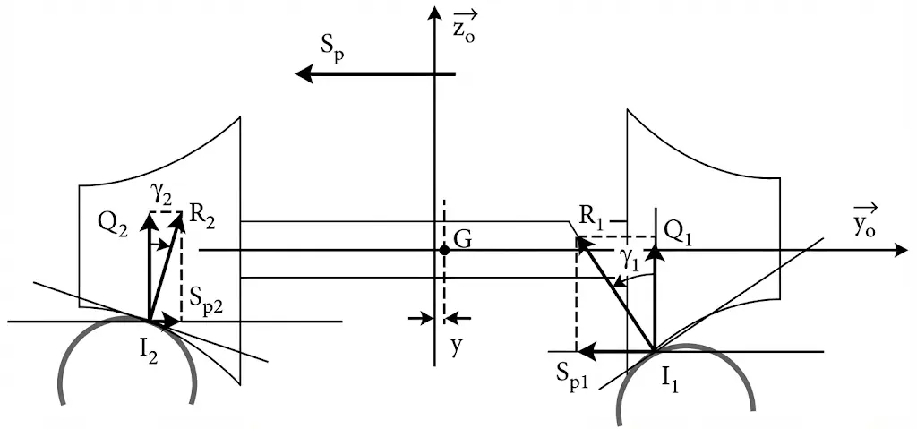 \(Q_{1}\), \(Q_{2}\) : Vertical components of reactions \(R_{1}\) and \(R_{2}\) at contact points \(\mathrm{I}_{1}\) and \(\mathrm{I}_{2}\), respectively.
\(\gamma_{1}\), \(\gamma_{2}\) : Angles formed by the horizontal plane and tangent planes at contact points \(\mathrm{l}_{1}\) and \(\mathrm{l}_{2}\), respectively (as \(\gamma_{1}\), \(\gamma_{2}\) are very small quantities, \(\tan \gamma_{1}=\gamma_{1}\) and \(\tan \gamma_{2}=\gamma_{2}\) apply).
\(Q_{1}\), \(Q_{2}\) : Vertical components of reactions \(R_{1}\) and \(R_{2}\) at contact points \(\mathrm{I}_{1}\) and \(\mathrm{I}_{2}\), respectively.
\(\gamma_{1}\), \(\gamma_{2}\) : Angles formed by the horizontal plane and tangent planes at contact points \(\mathrm{l}_{1}\) and \(\mathrm{l}_{2}\), respectively (as \(\gamma_{1}\), \(\gamma_{2}\) are very small quantities, \(\tan \gamma_{1}=\gamma_{1}\) and \(\tan \gamma_{2}=\gamma_{2}\) apply).
Rigorous determination of the above relationships is obtained through geometric analysis of wheel-rail interaction, assuming that: (i) the wheel possesses a conical shape with a constant radius curvature inclination, and (ii) the rail head presents a spherical surface of complementary curvature. From this geometric resolution, the following linear equations characterizing dynamic behavior are derived (Pyrgidis, 1990): \(\gamma_{1}=\gamma_{o}+\frac{\gamma_{e}}{R \cdot \gamma_{o}} \cdot y\) \(\gamma_{2}=-\gamma_{0}+\frac{\gamma_{e}}{R \cdot \gamma_{0}} \cdot y\) \(\gamma_{e}=\frac{R \cdot \gamma_{o}}{R-R^{\prime}}\)
R = Radius of curvature of the wheel tread \(R^{\prime}\)= Radius of curvature of the rail head running surface \(\gamma_{o}\): Inclination angle in the central equilibrium position.
Considering a symmetrical load distribution between both wheels, the total resulting gravitational force is obtained by:
\[S_{p}=S_{p 1}+S_{p 2}=2 Q_{o} \cdot \frac{\gamma_{e} \cdot y}{R \cdot \gamma_{o}}\]Alternatively, expressed in terms of curvature parameters:
I.7.3. Friction Forces
Straight Line Circulation
The friction forces emerging at the wheel-rail interface constitute a fundamental mechanism of dynamic interaction between vehicle and infrastructure. The longitudinal components of these friction forces are responsible for multiple detrimental effects: they promote progressive wear of the tread of both vehicle and rail, generate cyclic fatigue in constituent materials of the contact zone, produce significant acoustic emissions (rolling noise), and induce longitudinal vehicle oscillations.
To characterize friction forces resulting from the dynamics of a conventional wheel circulating on a straight path, Kalker’s linear theory is applied, providing the following analytical expressions:
\(X_{1}=-c_{11} \cdot\left(\frac{X^{\prime}}{V}-\frac{a}{2 \cdot V} \cdot \alpha^{\prime}-\frac{\gamma_{e}}{r_{o}} \cdot y\right)\) \(T_{1}=-c_{22} \cdot\left(\frac{y^{\prime}}{V}-\alpha\right)-c_{23} \cdot\left(\frac{\alpha^{\prime}}{V}-\frac{\gamma_{o}}{r_{o}}-\frac{\gamma_{e} \cdot y}{R \cdot \gamma_{o} \cdot r_{o}}\right)\) \(M_{1}=-c_{23} \cdot\left(\frac{y^{\prime}}{V}-\alpha\right)-c_{33} \cdot\left(\frac{\alpha^{\prime}}{V}-\frac{\gamma_{o}}{r_{o}}-\frac{\gamma_{e} \cdot y}{R \cdot \gamma_{o} \cdot r_{o}}\right)\)
\(X_{2}=-c_{11} \cdot\left(\frac{X^{\prime}}{V}+\frac{a}{2 \cdot V} \cdot \alpha^{\prime}+\frac{\gamma_{e}}{r_{o}} \cdot y\right)\) \(T_{2}=-c_{22} \cdot\left(\frac{y^{\prime}}{V}-\alpha\right)-c_{23} \cdot\left(\frac{\alpha^{\prime}}{V}+\frac{\gamma_{o}}{r_{o}}-\frac{\gamma_{e} \cdot y}{R \cdot \gamma_{o} \cdot r_{o}}\right)\) \(M_{2}=-c_{23} \cdot\left(\frac{y^{\prime}}{V}-\alpha\right)-c_{33} \cdot\left(\frac{\alpha^{\prime}}{V}+\frac{\gamma_{o}}{r_{o}}-\frac{\gamma_{e} \cdot y}{R \cdot \gamma_{o} \cdot r_{o}}\right)\)
 where:
\(\mathrm{X}_{1}, \mathrm{X}_{2}\) : Longitudinal friction forces applied on both wheels.
\(\mathrm{T}_{1}, \mathrm{~T}_{2}\) : Lateral friction forces applied on both wheels.
\(\mathrm{M}_{1}, \mathrm{M}_{2}\) : Turning moment on both wheels.
ro: wheel radius in its central equilibrium position
R: Radius of curvature of the wheel tread
x: Longitudinal displacement of the wheelset.
y : Lateral displacement of the wheelset.
\(\alpha\) : Wheelset angle of attack.
\(\varphi\) : Yaw angle of wheels and wheelset.
\(\mathrm{x}^{\prime}, \mathrm{y}^{\prime}, \alpha^{\prime}, \varphi^{\prime}\) : Derivatives of displacements \(\mathrm{x}, \mathrm{y}\),
of the angle of attack \(\alpha\), and of the yaw angle \(\varphi\).
\(\mathrm{c}_{11}\) : Kalker’s longitudinal coefficient.
c22: Kalker’s transverse coefficient.
\(\mathrm{c}_{23}, \mathrm{c}_{33}\) : Kalker’s spin coefficients.
where:
\(\mathrm{X}_{1}, \mathrm{X}_{2}\) : Longitudinal friction forces applied on both wheels.
\(\mathrm{T}_{1}, \mathrm{~T}_{2}\) : Lateral friction forces applied on both wheels.
\(\mathrm{M}_{1}, \mathrm{M}_{2}\) : Turning moment on both wheels.
ro: wheel radius in its central equilibrium position
R: Radius of curvature of the wheel tread
x: Longitudinal displacement of the wheelset.
y : Lateral displacement of the wheelset.
\(\alpha\) : Wheelset angle of attack.
\(\varphi\) : Yaw angle of wheels and wheelset.
\(\mathrm{x}^{\prime}, \mathrm{y}^{\prime}, \alpha^{\prime}, \varphi^{\prime}\) : Derivatives of displacements \(\mathrm{x}, \mathrm{y}\),
of the angle of attack \(\alpha\), and of the yaw angle \(\varphi\).
\(\mathrm{c}_{11}\) : Kalker’s longitudinal coefficient.
c22: Kalker’s transverse coefficient.
\(\mathrm{c}_{23}, \mathrm{c}_{33}\) : Kalker’s spin coefficients.
Circulation in Curves
In the context of movement in track curvature, friction mechanisms undergo significant modifications compared to the straight line case. For a conventional axle transiting through a curved infrastructure section, Kalker’s linear theory provides the following analytical expressions corrected to capture horizontal curvature effects:
\[\begin{aligned} & X_{1}=-c_{11} \cdot\left(-\frac{\gamma_{e}}{r_{o}} \cdot y-\frac{a}{2 \cdot V} \cdot \alpha^{\prime}+\frac{a}{2 \cdot R_{c}}\right) \\ & X_{2}=-c_{11} \cdot\left(+\frac{\gamma_{e}}{r_{o}} \cdot y+\frac{a}{2 \cdot V} \cdot \alpha^{\prime}-\frac{a}{2 \cdot R_{c}}\right) \\ & T_{1}=-c_{22} \cdot\left(\frac{y^{\prime}}{V}-\alpha\right)-c_{23} \cdot\left(\frac{\alpha^{\prime}}{V}-\frac{1}{R_{c}}-\frac{\gamma_{o}}{r_{o}}-\frac{\gamma_{e} \cdot y}{R \cdot \gamma_{o} \cdot r_{o}}\right) \\ & T_{2}=-c_{22} \cdot\left(\frac{y^{\prime}}{V}-\alpha\right)-c_{23} \cdot\left(\frac{\alpha^{\prime}}{V}-\frac{1}{R_{c}}+\frac{\gamma_{o}}{r_{o}}-\frac{\gamma_{e} \cdot y}{R \cdot \gamma_{o} \cdot r_{o}}\right) \\ & M_{1}=-c_{23} \cdot\left(\frac{y^{\prime}}{V}-\alpha\right)-c_{33} \cdot\left(\frac{\alpha^{\prime}}{V}-\frac{\gamma_{o}}{r_{o}}-\frac{1}{R_{c}}-\frac{\gamma_{e} \cdot y}{R \cdot \gamma_{o} \cdot r_{o}}\right) \\ & M_{2}=-c_{23} \cdot\left(\frac{y^{\prime}}{V}-\alpha\right)-c_{33} \cdot\left(\frac{\alpha^{\prime}}{V}+\frac{\gamma_{o}}{r_{o}}-\frac{1}{R_{c}}-\frac{\gamma_{e} \cdot y}{R \cdot \gamma_{o} \cdot r_{o}}\right) \end{aligned}\]Rc: radius of curvature of horizontal alignment.
In the particular motion regime in small radius curves, where circulation speed approximates the equilibrium speed corresponding to that radius, dynamic behavior can be significantly simplified. In such conditions, inertia and damping forces result negligible compared to track elastic stiffness forces. Additionally, when axle spin effect is ignored, equations reduce to the following forms, capturing essential behavior aspects without excessive mathematical complexity:
\[\begin{aligned} & X_{1}=-c_{11} \cdot\left(-\frac{\gamma_{e}}{r_{o}} \cdot y+\frac{a}{2 \cdot R_{c}}\right) \\ & X_{2}=-c_{11} \cdot\left(+\frac{\gamma_{e}}{r_{o}} \cdot y-\frac{a}{2 \cdot R_{c}}\right) \\ & T_{1}=T_{2}=-c_{22} \cdot\left(\frac{y^{\prime}}{V}\right) \end{aligned}\]As evidenced in the simplified analysis presented, longitudinal friction forces generate horizontal wheelset rotation, which in combination with lateral friction forces activates the sinusoidal oscillation phenomenon (hunting) in bogie axles, causing persistent lateral vibrations and oscillations.
Fundamentally, friction forces originate as a response to deviations between the wheel rolling direction and the actual axle displacement. Such deviations occur both upon transverse displacements “y” of the axle and upon variations in the angle of attack “a” relative to the equilibrium position. Consequently, to mitigate friction forces it results essential to focus on causative parameters: track geometric irregularities.
Mitigating measures contributing to friction force reduction include:
A. Wheel reprofiling and turning at regular intervals, ensuring maintenance of optimal geometries.
B. Careful selection of fundamental bogie constructive characteristics: specific wheel reprofiling, nominal rolling diameter, primary suspension stiffness, and bogie wheelbase.
C. Adoption of modern bogie technologies concordant with operational requirements of the railway network.
Specialized technical aspects of friction forces:
- Presence or absence of longitudinal and lateral friction components fundamentally depends on the connection mode between wheel and axle.
- Turning moment generation is conditioned by the geometric relationship between wheel rolling plane and its rotation axis.
The following table synthesizes the wheel-rail contact force repertoire for different railway axle technologies (materialized or theoretically proposed) (Frederich, 1985):
| Technology | Schematic Representation | Sp | T | x | M |
|---|---|---|---|---|---|
| Conventional axles - Variable conicity wheels |  |
Yes | Yes | Yes | Yes |
| Axles with independently rotating wheels - Variable conicity wheels |  |
Yes | Yes | No | Yes |
| Articulated axles - Variable conicity wheels | 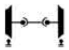 |
Yes | No | Yes | Yes |
| Conventional axles - Cylindrical wheels | 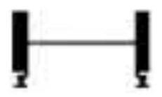 |
No | Yes | Yes | No |
| Conventional axles - Constant conicity wheels | 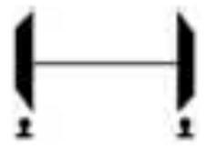 |
No | Yes | Yes | Yes |
| Independently rotating wheels - Variable conicity wheels | 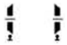 |
Yes | No | No | Yes |
| Axles with independently rotating wheels - Inclined variable conicity wheels | 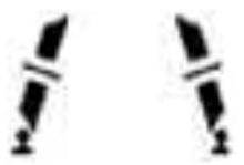 |
Yes | No | No | No |
| Conventional axles - Inclined variable conicity wheels | 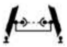 |
Yes | Yes | Yes | No |
Frederich, F. 1985, Possibilités inconnues et inutilisées du contact rail-roue, Rail International, Brussels, November 1985 pp. 33-40
A relevant technological aspect to reduce unfavorable effects of longitudinal friction forces consists of eliminating the rigid coupling traditionally joining the two wheels of the same axle. This modification allows each wheel to rotate at an independent angular speed, while maintaining the kinematic condition that both wheels circulate without relative sliding regarding their respective contact lines:
\[\omega_{1} \cdot r_{1}=\omega_{2} \cdot r_{2}=V\]where: \(\omega_{1}, \omega_{2}\) : Angular speeds of the two wheels. \(r_{1}, r_{2}\) : Their rolling radii.
This guarantees rolling of both wheels without friction and elimination of longitudinal friction forces. Technology of bogies with independently rotating wheels is based on this logic.
I.8.4. Crosswind Forces
Atmospheric wind action constitutes an environmental stress of significance in railway systems operation, especially on viaducts, mountainous zones, and exposed coastal areas. When transverse winds of considerable magnitude prevail, a lateral force \(\boldsymbol{H}_{\boldsymbol{w}}\) is transmitted through the vehicle body and structure towards wheelsets, and from these towards rail running surface. This force is characterized as quasi-static in nature, adopting a direction coincident with prevailing wind. The initial application point is located at the geometric center of the body lateral projection. The calculation expression quantifying this stress comes from vehicular aerodynamics (Hibino et al., 2010): \(H_{w}=\frac{1}{2} \cdot \rho \cdot S_{2} \cdot V_{w}^{2} \cdot K_{2}\) specifying parameters as follows: \(\mathrm{H}_{\mathrm{w}}\) : Magnitude of transverse force exerted by wind (expressed in Newtons) \(\mathrm{V}_{\mathrm{w}}\) : Wind speed (expressed in meters per second) \(\rho\) : Air volumetric density (expressed in kilograms per cubic meter) \(\mathrm{S}_{2}\) : Vehicle lateral projection area perpendicular to wind flow (expressed in square meters) \(\mathrm{K}_{2}\) : Lateral force aerodynamic coefficient (dimensionless parameter dependent on body external geometry)
The transverse wind force \(H_{w}\) represents an undesirable stress, generating multiple detrimental effects: promotes excessive transverse displacements of wheelsets towards leeward side, increases risk of contact between wheel flanges and rails, and fundamentally amplifies vehicle overturning mechanism activation potential.
To counteract intense crosswind effects, the following mitigation measures can be implemented:
- Installation of windbreak barrier or screen systems in track sections particularly exposed to severe weather
- Operational restrictions: speed reduction or temporary suspension of circulation in zones of high exposure to extreme crosswinds
I.8.5. Unbalanced Centrifugal Force
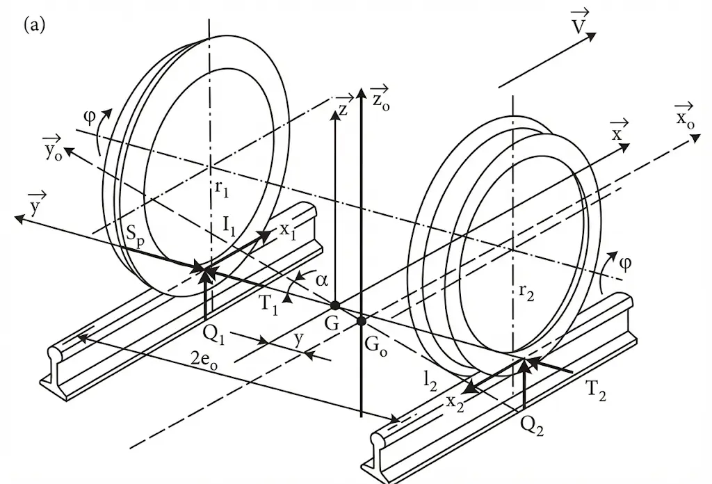
When a vehicle of mass \(\boldsymbol{m}\) circulates at a speed \(\boldsymbol{V}\) in a curve whose radius of curvature is \(\boldsymbol{R}\), the vehicle center of gravity generates centrifugal force \(\boldsymbol{F}_{\boldsymbol{c}}\), pushing the vehicle towards curve outer side (figure):
\[F_{c}=m \cdot \alpha_{c}=\frac{m \cdot V^{2}}{R}\]Due to track cant \(\mathbf{z}_{\boldsymbol{p}}\), weight transverse component (in opposite direction) and centrifugal force act simultaneously. Being: \(\quad I=\alpha_{s c} \cdot \frac{a}{g}\) The difference between these forces is the unbalanced centrifugal force \(\boldsymbol{F}_{\boldsymbol{n} \boldsymbol{c}}\). At wheelset level and, consequently, rail running surface, the following applies:
\[F_{c, S C}=m \cdot \alpha_{S C}=\frac{Q}{g} \cdot \alpha_{S C}=\frac{Q}{g} \cdot\left(\frac{V^{2}}{R}-\frac{g \cdot z_{p}}{a}\right)=\frac{Q \cdot I}{a}\]Vehicle speed \(\boldsymbol{V}\) increase, as well as curvature radius \(\boldsymbol{R}\) decrease and cant \(\mathbf{z}_{\boldsymbol{p}}\) decrease contribute to residual centrifugal acceleration increase.
\(\boldsymbol{F}_{\boldsymbol{c}, \boldsymbol{s} \boldsymbol{c}}\) is considered a quasi-static force and is always undesirable, as it not only causes wheelset displacement (flange contact risk), but also transverse dynamic passenger comfort problems. Besides, it aids vehicle derailment mechanism. However, traffic reasons such as coexistence of low and high-speed trains on same track and risk of wheelset transverse sliding towards inner rail make adoption of a cant lower than equilibrium cant (theoretical cant) indispensable, causing residual centrifugal acceleration appearance.
For example, when \(Q=18 t, V=150 \mathrm{~km} / \mathrm{h}, R=1,500 \mathrm{~m}, g=9.81 \mathrm{~m} / \mathrm{s}^{2}\), \(a= 1.50 m\) and \(z_{p}=130 m m\), then \(F_{c, s c}=5.6 k N\) and \(\alpha_{s c}=0.307 m / s^{2}\).
To reduce residual centrifugal force, following measures can be applied:
- Rational choice of curve geometric data (cant deficiency and excess).
- Use of tilting trains.
I.8.6. Total Transverse Force Transmitted from Vehicle to Rail
According to Alias (1977) and Profillidis (1995), total transverse force H (in t) transmitted from vehicle to rail is calculated applying following empirical formula:
\[H=H_{o}+H_{a}=a_{i} \cdot\left(\frac{Q \cdot I}{a}\right)+\left(\frac{Q \cdot V}{1,000}\right)\]where: I: Cant deficiency (in case of movement along curved track sections) or transverse track defect or twist (in case of movement in straight trajectory) (in mm). Q: Axle load (in t). V: Running speed (in km/h). a: distance between rail axes in mm. \(a_{i}\) : Coefficient indicating unequal centrifugal force distribution between two axles of a bogie (values 1-1.1) (Montagné, 1975).
First term of equation refers to quasi-static forces and, concretely, to residual centrifugal force. Second term refers to random dynamic forces derived from track alignment irregularities and movements of vehicle itself, or its bogies, causing instability above a critical speed (forces due to vehicle oscillations, friction forces, gravitational forces, etc.) (Montagné, 1975).
I.8.7. Forces Due to Vehicle Oscillations
These transverse dynamic loads \(P_{\text {dyn, whose causes are similar to }}\) those of vertical dynamic loads, confer supplementary transverse accelerations to different vehicle parts. To solve problem, it is precise to eliminate track defects and apply rail grinding.
I.8.8. Guiding Forces
When transverse displacement of a railway wheelset reaches a magnitude equal to nominal clearance \(\boldsymbol{J}\) available between wheel flange and neighboring rails, flange lateral protruding zone enters direct contact with rail inner face (see reference schematic figures). At flange-rail contact point, transverse dynamic loads of generally considerable magnitude act. These forces are termed “guiding forces” \(\boldsymbol{F}_{\boldsymbol{j}}\) ( \(\mathrm{j}=1\) or 2, referring to each of two axle wheels).
Operational consequences of guiding forces existence constitute a set of significant negative impacts affecting simultaneously passengers, rolling stock and railway infrastructure:
- Marked degradation of dynamic comfort perceived by passengers, manifested through transverse acceleration increases and perceptible lateral “jerks”
- Considerable rolling noise generation, with environmental impact in adjacent urban zones
- Promotion of accelerated wear of running surfaces of both wheels and rails (abrasion of flanges and rail heads)
- Significant increase of structural fatigue in bogie components
- Potential triggering of derailment by track lateral sliding under repeated guiding loads
- Risk of derailment by wheel climbing or mounting over rail head when guiding forces reach critical magnitudes
Consequently, from railway safety engineering perspective, it is of utmost importance to avoid, whenever technically feasible, wheel flange contact with rails during normal vehicle operation.
To minimize and control guiding forces magnitude, several categories of mitigating measures can be adopted:
- Careful and rational selection of fundamental bogie design parameters: specific wheel geometric profile, nominal rolling diameter, stiffness and damping characteristics of bogie primary suspension, and bogie wheelbase separation distance
- Adoption of modern and advanced bogie technologies optimizing dynamic behavior and being concordant with specific railway network operational characteristics
- Controlled widening of lateral clearance \(J\) in curved track segments of very small radius ( \(Rc<150-200 \mathrm{~m}\) ), allowing greater transverse freedom before contact
- Application of high-performance lubrication on rail inner face in curved segments, reducing flange friction and transmitted lateral forces
From an analytical and methodological perspective, guiding force \(F\) presents statistical characteristics (stochastic nature), implying its instantaneous magnitude varies randomly in time (Profillidis, 2014). Magnitude of this force depends on numerous parameters interacting non-linearly. Consequently, for most practical applications accurate calculation of its value is achieved through numerical approximations, predominantly through dynamic simulation methodologies:
a) In situ measurements along rail using specialized dynamometers mounted on instrumented vehicle wheels b) Computational simulation models, of which a variety exists in professional market (SIMPACK, UMLAB, Vampire Pro, Adams/Rail, etc.), widely used by both industry and research community.
Guiding forces \(F_{j}\) are derived as result of algebraic combination of all individual transverse force components interacting in wheelset (each component obtained from simulation model):
\[F_{j}= \pm\left(T_{1}+T_{2}\right) \pm S_{p} \pm F_{s c} \pm F_{r e s}\]Terms integrating this relationship are defined as follows: \(\mathrm{T}_{1}, \mathrm{~T}_{2}\) : Lateral components of friction forces applied at contact points of each wheel respectively \(\mathrm{S}_{\mathrm{p}}\) : Total resulting gravitational (restoring) force of both wheels \(\mathrm{F}_{\mathrm{nc}}\) : Unbalanced centrifugal force transmitted to wheelset Fres: Lateral reaction forces produced by elastic elements (springs) of bogie primary suspension.
For particular case of wheelset derailment, when wheelset angle of attack reaches very significant magnitudes ( \(\alpha \geq 5\) rad), following simplified relationship applies:
\[F_{1}=H+Y_{2}\]where parameters are defined as follows: \(F_{1}\) : Guiding force applied at flange-rail contact point of wheel in critical derailment state H: Total lateral force transmitted from vehicle to rail (quantified at wheelset level)
\[Y_{2}=Q_{2} \cdot \tan \left(\gamma_{2}+\rho_{2}\right)\]Q2: Static vertical load of wheel 2 \(\gamma_{2}\) : Wheel-rail contact angle (i.e., angle between wheel rolling generatrix and horizontal plane) \(\rho_{2}\) : Static friction angle at wheel-rail interface of wheel 2
Empirical expression relating friction angle with track curvature radius is (Amans and Sauvage, 1969; Joly, 1983):
\[\tan \left(\gamma_{2}+\rho_{2}\right)=\frac{135}{(150+R)}\]Numerical value of \(\tan \rho_{2}\) varies as function of prevalent climatic and environmental conditions, typically adopting values in range 0.15 to 1.25 (Amans and Sauvage, 1969). For standard case of rails with 1:40 inclination one has \(\gamma_{2}=0.02\) rad.
This relationship can be rewritten approximately as:
\[\frac{135}{\left(150+R_{c}\right)} \approx \mu\]where \(\mu\) represents adherence dimensionless coefficient (Joly, 1983).
Rc: Horizontal alignment radius of curvature (expressed in meters).
Chapter II. Derailment
Fundamental Concept: The term “derailment” constitutes the description of a critical event characterizing irreversible loss of contact between at least one railway vehicle wheel and working or rolling surface of rail head, resulting in unintentional exit of rolling stock from its designated path.
Railway vehicle derailments can originate and manifest as consequence of three differentiated physical mechanisms:
- Involuntary lateral displacement or shifting of track itself
- Uncontrolled overturning and tilting of vehicle
- Climbing or mounting of one or several wheels over rail head
In terms of classification by origin, causes provoking derailments can be:
- Of nature internal to system (excessive forces generated by vehicle on infrastructure, circulation at speeds higher than permitted, deterioration of rolling stock quality, deficiencies in track geometric design, embankment erosion or collapse, etc.) or
- Of nature external to system (operation and driving errors, adverse weather events such as extreme winds, presence of obstacles, sabotage, etc.).
II.0.1. Derailment Due to Vehicle Overturning
Phenomenon of derailment induced by vehicle overturning constitutes contact loss mechanism capable of manifesting both during circulation in curved track segments and during movement in rectilineal infrastructure sections.
Verification of overturning derailment in curved track segments
Overturning can occur following two distinct trajectories: towards curve outer side or towards same inner side.
Overturning directed towards curve exterior (Esveld, 2001) may be due to multiple concurrent factors:
- Significant cant insufficiency with respect to passage speed Vp and path curvature radius, producing increase in residual lateral centrifugal force magnitude Fnc.
- Presence of aerodynamic forces generated by crosswinds Hw directed towards curve outer side.
- Unequal vertical vehicle mass distribution between its two lateral wheels, particularly when overload exists on outer side (Q1 > Q2). All these factors combined generate destabilizing moments driving vehicle overturning towards outer rail.
Overturning directed towards curve interior may be due to:
- Aerodynamic forces generated by crosswinds \(\mathrm{H}_{\mathrm{w}}\) directed towards curve inner side.
- Immobility or complete stop of vehicle ( \(V=0\) ) located in curved track segment with elevated cant \(\mathrm{z}_{\mathrm{p}}\).
- Reduced or insufficient axle loads.
- Displacement or migration of vehicular mass towards curve inner side.
In these cases, force moments driving vehicle overturning towards inner rail are generated, finally precipitating derailment.
Evaluation and verification of overturning derailment risk can be carried out through two approaches: rigorous analytical formulations or empirical methodologies based on experience.
II.0.2. Use of Analytical Relations
Evaluation procedure is based on rigorous analysis of moments of all forces acting on vehicle, considering its rotation around critical contact point located on rail head where overturning starts (see reference figure). For this evaluation fundamental equation proposed by Rivier (Rivier, 1984/85) is applied:
\[V_{\text {der }, o v}^{2}=\frac{R \cdot g \cdot\left(\frac{z_{p}}{a}+\frac{a}{2 h_{K B}}\right)}{1-\left(\frac{z_{p}}{a} \cdot \frac{a}{2 h_{K B}}\right)}\]where parameters are defined: \(V_{\text {der.ov:}}\) Critical speed from which overturning derailment occurs. \(h_{\mathrm{kB}}\) : Height or vertical distance between vehicle mass center of gravity and rail contact surface. g: Terrestrial gravity acceleration. a: Transverse distance between vertical symmetry axes of both rails.
II.0.3. Derailment Due to Vehicle Overturning
Use of Empirical Formulations
This evaluation method is applicable solely when center of gravity height satisfies condition \(h_{\mathrm{kB}}>2.25\) m and is restricted exclusively to cases where overturning is oriented towards road infrastructure exterior (Amans and Sauvage, 1969).
For overturning derailment phenomenon to occur, following limit condition must be met: \(\alpha_{s c, \max }>\frac{g}{3}\)
where: \(\alpha_{s c, m a x}\) : Maximum uncompensated lateral acceleration vehicle can withstand.
Additionally, following mathematical relations apply: \(\alpha_{s c}=\frac{V^{2}}{R}-\frac{g \cdot z_{p}}{a} \quad \alpha_{s c}=g \cdot \frac{I}{a} \quad I=\frac{a \cdot V^{2}}{g \cdot R}-z_{p}\)
From analysis of these equations it can be deduced that for occurrence of derailment directed towards track exterior by overturning effect, following fundamental condition must be satisfied:
\[\alpha_{s c}=g \cdot \frac{I}{a}>\frac{g}{3} \rightarrow I>\frac{a}{3} \rightarrow V>V_{d e r, o v}=\sqrt{R \cdot g \cdot\left(\frac{1}{3}+\frac{z_{p}}{a}\right)}\]II.0.4. Verification of Overturning Derailment - Movement in Straight Track Segments
In context of vehicle movement in straight horizontal infrastructure alignments, this specific derailment type can manifest solely under extremely severe transverse aerodynamic force conditions, displacement direction being always concordant with acting wind direction.
II.0.5. Using Analytical Relations
This verification procedure is grounded in balanced analysis of all acting moments: A. Moment generated by crosswind aerodynamic force, and B. Moment resulting from total vehicle weight, both considered regarding critical contact point on rail head around which overturning would occur.
For this evaluation following fundamental mathematical equations are employed: \(M_{t} \cdot g \cdot \frac{a}{2}=q_{o}^{*} \cdot H_{w} \quad H_{w}=\frac{1}{2} \cdot \rho \cdot S_{2} \cdot V_{w}^{2} \cdot K_{2}\)
\[V_{w}=\sqrt{\frac{M_{t} \cdot g \cdot a}{q_{o}^{*} \cdot \rho \cdot S_{2} \cdot K_{2}}}\]where parameter meanings are specified: Mt: Total mass of structure and railway vehicle content (expressed in kilograms). \(\mathrm{H}_{\mathrm{w}}\) : Magnitude of transverse or lateral aerodynamic force generated by wind (expressed in Newtons). \(\mathrm{V}_{\mathrm{w}}\) : Atmospheric wind speed in m/sec. \(\rho\) : Air volumetric density (kg/m³). \(\mathrm{S}_{2}\) : Vehicle lateral projection area exposed to aerodynamic forces (expressed in m²). \(\mathrm{K}_{2}\) : Lateral aerodynamic resistance dimensionless coefficient (parameter dependent on vehicle lateral surface geometry). \(\mathrm{q}^{*} \circ\left(=1.25 \mathrm{q}_{o}\right)\) : Compensated effective height of transverse aerodynamic force application point, measured from rails running surface (expressed in meters).
II.0.6. Derailment by Track Lateral Displacement
In derailment mechanism associated with track lateral displacement, set of structural elements forming road superstructure (rails, sleepers, fastening systems) experience significant magnitude involuntary lateral movement under influence of excessive transverse forces, finally precipitating derailment of one or multiple vehicles circulating in train.
Derailment by track lateral displacement occurs when following condition is met: \(H>H_{R}\)
where: H: Total lateral force transferred and transmitted from vehicle towards rail. \(\mathrm{H}_{\mathrm{R}}\) : Lateral resistance capacity of complete track structure.
This specific derailment type is attributable exclusively to causes and factors internal to railway system, constituting most frequently observed derailment mechanism in operative practice.
Total lateral force H (expressed in tons) can be calculated applying following consolidated empirical formula: \(H=H_{o}+H_{a}=a_{i} \cdot\left(\frac{Q \cdot I}{a}\right)+\left(\frac{Q \cdot V}{1,000}\right)\)
II.0.7. Derailment by Track Lateral Displacement - Resistance Calculation
Regarding systematic calculation of infrastructure lateral resistance \(\mathrm{H}_{\mathrm{R}}\) multiple mathematical formulations have been developed and proposed in specialized literature (ORE, 1984; Amans and Sauvage, 1969; Prud’homme, 1967). For reference and practical application, most used formulations are presented below (\(\mathrm{H}_{\mathrm{R}}\) is calculated in tons):
Prud’homme Resistance Criterion
\[H_{R}=0.85 \cdot\left(1+\frac{Q}{3}\right)\]where: \(\mathrm{H}_{\mathrm{R}}\) : Track lateral resistance capacity (expressed in tons). Q: Vertical load magnitude per railway axle (in tons).
This equation (applied with corrective factor 0.85) incorporates implicitly track horizontal alignment effect and thermal stresses acting on rail elements, although assuming implicitly a track not fully stabilized through consolidation.
Derailment by Track Lateral Displacement: Alternative Empirical Formulas
For infrastructures with concrete sleepers: \(H_{R}=0.6 \cdot(Q+6) \cdot\left(1-0.4 \cdot e^{\frac{T_{t}}{60,000}}\right)\)
where: Q: Vertical load applied per axle (in tons). Tt: Accumulated traffic volume circulated (in tons).
For a track fully stabilized through traffic (\(\mathrm{T}_{\mathrm{t}}=\infty, e^{\frac{T_{t}}{60,000}}=0\)) previous equation reduces to: \(H_{R}=0.6 \cdot Q+3.6\)
For a track not yet stabilized (\(\mathrm{T}_{\mathrm{t}}=0, e^{\frac{T_{t}}{60,000}}=1\)) equation transforms into: \(H_{R}=0.36 \cdot Q+2.16\)
For infrastructures with wooden sleepers: \(H_{R}=0.5 \cdot(Q+4) \cdot\left(1-0.4 \cdot e^{\frac{T_{t}}{60,000}}\right)\)
For fully stabilized track (\(\mathrm{T}_{\mathrm{t}}=\infty\)): \(H_{R}=0.5 \cdot Q+2\)
For unstabilized track (\(\mathrm{T}_{\mathrm{t}}=0\)): \(H_{R}=0.3 \cdot Q+1.2\)
II.0.8. Derailment by Track Lateral Displacement - Formula Application
If following relations are incorporated in analysis: \(\quad z_{t, \text { max }}(mm)=11.8 \cdot \frac{V_{\text {max }}^{2}(Km/h)}{R(m)} \quad\) and \(\quad I=z_{t, \text { max }}-z_{p}\)
And considering mathematical expressions: \(H_{R}=0.6 \cdot(Q+6) \cdot\left(1-0.4 \cdot e^{\frac{T_{t}}{60,000}}\right) \quad H_{R}=0.5 \cdot Q+2 \quad H=a_{i} \cdot\left(\frac{Q \cdot I}{a}\right)+\left(\frac{Q \cdot V}{1,000}\right)\)
Together with hypothesis of uniform centrifugal force distribution between both bogie axles ( \(\mathrm{a}_{\mathrm{i}}=1\) and \(\mathrm{a}=1500\)mm), it is possible to establish, based on critical condition \(\mathrm{H}>\mathrm{H}_{\mathrm{R}}\), that critical derailment speed \(\mathrm{V}_{\text {der.dis }}\) from which derailment by lateral displacement occurs (for concrete or wooden sleepers in fully stabilized track) comes given by polynomial equations:
Track with concrete sleepers: \(\left(11.8 \cdot \frac{Q}{R}\right) \cdot V_{\text {der,dis }}^{2}+1.5 \cdot Q \cdot V_{\text {der,dis }}-Q \cdot\left(z_{p}+900\right)-5400=0\)
Track with wooden sleepers: \(\left(11.8 \cdot \frac{Q}{R}\right) \cdot V_{\text {der,dis }}^{2}+1.5 \cdot Q \cdot V_{\text {der,dis }}-Q \cdot\left(z_{p}+750\right)-3000=0\)
where: \(Q(t), R(m), \mathrm{z}_{\mathrm{p}}(\mathrm{mm})\), and \(V_{\text {der.dis }}(\mathrm{km} / \mathrm{h})\)
In straight track horizontal alignments, where cant is absent, parameter I (representing cant deficiency) assimilates to alignment transverse defect or twist. In ideal conditions where transverse defect is null, theoretically derailment risk by lateral displacement does not exist. If we equal \(\mathrm{I}=0\), previous equations transform:
Track with concrete sleepers: \(V_{\text {der,dis }}=600+\frac{3600}{Q}\)
Track with wooden sleepers: \(V_{\text {der,dis }}=500+\frac{2000}{Q}\)
For a standard load of \(Q=22.5\) t, \(V_{\text {der.dis }} \geq 760\) km/h is required (for concrete sleepers) and \(V_{\text {der.dis }} \geq 589\) km/h (for wooden sleepers) for lateral displacement derailment to occur.
Taking into account exposed analysis, to minimize and effectively reduce risk of derailment by track lateral displacement, strategies pointing to following must be adopted:
A. Reduce magnitude of lateral force H transferred from vehicle towards infrastructure or B. Increase transverse resistance capacity of track \(\mathrm{H}_{\mathrm{R}}\) or C. Implement combined measures addressing both aspects simultaneously.
Regarding force H, parameters affecting it derive directly or indirectly from fundamental equation:
\[H=a_{i} \cdot\left(\frac{Q \cdot I}{a}\right)+\left(\frac{Q \cdot V}{1,000}\right)\]In relation to transverse resistance \(\mathrm{H}_{\mathrm{R}}\), following design and construction parameters significantly increase its value:
- Use of prefabricated concrete sleepers of high mass
- Employment of continuous welded rails of high mass per unit length
- Fastening systems with elastic components
- Track fully stabilized through consolidated traffic
- Slab track infrastructures
- Track bed substructure in excellent state
In particular case of ballasted infrastructures:
- Considerable width of ballast lateral support zone
- Generous thickness of ballast layer
- High degree of compaction and hardness of granular material
- Infrequent tamping cycles preserving consolidation
II.0.9. Derailment by Wheel Flange Climbing
For occurrence of flange climbing derailment to be possible it is necessary that contact between flange and rail inner face has previously occurred, generating consequently guiding forces (F) driving climbing.
At contact point between wheel flange and rail inner face (see reference figures), wheel exerts guiding force \(F_{1}\) on rail, together with vertical wheel load \(Q_{1}\). In turn, rail reacts with vertical force \(N_{1}\) and lateral friction force \(\mathrm{T}_{1}\) (which during sliding acquires Coulomb friction force value).
In operative practice, flange climbing derailment occurs when resultant of all force projections on vertical action axis (derailment force axis) orients upwards, and time during which this resultant force acts is sufficiently prolonged to allow wheel to ascend and overcome rail head height.
Derailment can occur when significant vertical unloading of wheel about to derail exists simultaneously with vertical overload of opposite wheel of same axle.
This phenomenon is typically observed during low speed circulation in small radius curves presenting high cant and track twist values.
Normally this derailment modality is produced by causes external to system (switch malfunction and misalignment, etc.). Most derailments in switch zones and crossings obey multiple concurrent causes. Derailment can manifest in turnouts when developed centrifugal force reaches very significant magnitudes (in straight turnouts no alignment cant exists) and simultaneously track lateral resistance is high (generating sudden derailments) (Centre for Advanced Maintenance Technology, 1998).
Risk of derailment by flange climbing increases significantly when concur:
- Increase in guiding force magnitude
- Greater temporal duration of guiding force application
- Increase in wheel-rail friction coefficient (in rain conditions risk is lower)
- Greater wheelset inclination angle
- Decrease in contact angle between rail and wheel flange
- Important vertical unloading of derailed wheel simultaneously with overload of opposite wheel
Specific time is required during which derailed wheel travels certain distance on track, typically some meters. This distance is termed “flange climbing distance” and is defined as distance traveled from instant total guiding force value acts until moment angle of contact between flange and rail reaches \(26.6°\) (Dos Sandos et al., 2010).
To carry out verification and evaluation of derailment risk by flange climbing following methodologies and technical criteria can be employed:
Criteria based on evaluation of relation \(F_{1}\) / \(Q_{1}\)
Derailment is avoided when following fundamental condition is met:
\[\frac{F_{1}}{Q_{1}}<K_{d}\]where: \(\mathrm{K}_{\mathrm{d}}\) : Critical derailment factor (specifically related to flange climbing). Q1: Static vertical load of wheel being evaluated under derailment risk (assuming wheel 1). \(\mathrm{F}_{1}\) : Applied guiding force magnitude.
Technical criteria evaluating this relationship are widely documented in specialized literature (FP7, 2011; Iwnicki, 2006; Ishida and Matsuo, 1999; Alias, 1977; Profillidis, 2005) and include non-exhaustively following:
- Nadal Criterion (presupposes wheel-rail angle of attack is not exactly zero)
- Weinstock Criterion
- Chartet Criterion (applicable for angles of attack of \(\alpha>1°\))
- Derailment criterion for high angles of attack (\(\alpha>5\) mrad)
In accordance with data reported in specialized bibliography (FP7, 2011; Iwnicki, 2006; Ishida and Matsuo, 1999; Umdrucke zur Grundvorlesung, 2002/2003):
- In Japan and Western Europe typically \(\mathrm{K}_{\mathrm{d}}=0.8\) is employed
- In South American countries \(\mathrm{K}_{\mathrm{d}}=1.0\) is adopted
- In China limit value is considered \(\mathrm{K}_{\mathrm{d}}=1.0\) while risk limit corresponds to \(\mathrm{K}_{\mathrm{d}}=1.2\)
Empirical formula for calculation of critical climbing derailment speed
By equating following expressions (Rivier, 1984/85): \(F_{C, S C}=\frac{Q}{4} \quad F_{C, S C}=\frac{Q}{g} \cdot\left[\frac{V^{2}}{R}-\frac{g \cdot z_{p}}{a}\right]\)
Expression obtained: \(V_{\text {der }, wcl}=\sqrt{R \cdot g \cdot\left(\frac{z_{p}}{a}+\frac{1}{4}\right)}\)
where: \(V_{\text {der.wcl:}}\) Critical speed from which derailment by flange climbing occurs.
Expressions \(F_{c, S c}=\frac{Q}{4}\) and \(\mathrm{V}_{\text {der.wcl }}\) were proposed by Professor Rivier of Swiss Federal Institute of Technology in Lausanne, grounding in pure experimental evidence. These expressions correspond to most unfavorable and critical conditions for occurrence of flange climbing derailment.
II.0.10. Derailment by Gauge Widening or Rail Lateral Overturning
In this derailment mechanism, interaction of large lateral forces transmitted by wheels on rails in curved infrastructure segments can generate significant lateral displacements of both rails and/or rail head overturning, frequently resulting in fall of wheel not having derailed between two rail heads (see reference figures) (Iwnicki, 2006; Blader, 1990).
Longitudinal gauge wear constitutes another cause contributing to space increase between rails.
To carry out verification of derailment risk caused by gauge widening following formulation is used (see figures): \(G \geq B+e+w_{wh}\)
where: G: Track gauge measured between rail inner heads. e: Wheel flange thickness. B: Distance between wheels (measured between inner surfaces of both wheels). \(w_{wh}\) : Wheel width on its tread.
For verification of derailment risk caused by rail head overturning following formulation applies (Iwnicki, 2006): \(F>Q \cdot \frac{d_{i}}{h_{r}}\)
where: \(\mathrm{h}_{\mathrm{r}}\) : Total rail section height. d: Maximum distance measured from rail foot (base) edge to application point of resultant of all total vertical loads acting on rail.
II.0.11. Derailment in Switches and Turnouts
In straight turnouts and specifically in turnout circular section, no cant is provided in track alignment ( \(\mathrm{z}_{\mathrm{p}}=0\)), nor gauge widening is implemented, nor smooth transition curves exist.
In event train enters turnout with speed considerably higher than allowed by horizontal alignment curvature radius, resulting centrifugal force increase can precipitate derailment by flange climbing.
In straight turnouts following fundamental relationship applies: \(z_{p}=z_{t}-I=0 \quad \text{being:} \quad z_{t}=11.8 \cdot \frac{V^{2}}{R}\)
where: \(\mathrm{z}_{\mathrm{t}}\) : Theoretical or equilibrium cant \(=11.8 V^2 / R\) (in mm) I: Cant deficiency (expressed in mm) V: Train passage speed through turnout (in km/h) \(\mathrm{Z}_{\mathrm{p}}\) : Real track cant in turnout (in mm) R: Turnout trajectory curvature radius (in meters)
From substitution of two previous equations it concludes: \(V=0.29 \cdot \sqrt{R \cdot I}\)
Based on above and assuming \(\mathrm{Z}_{p}=0\), it is possible to calculate critical derailment speed for various derailment mechanisms, transforming as follows:
Derailment by vehicle overturning: \(V_{der,ov}>\sqrt{R \cdot \frac{g}{3}} \quad V_{der,ov}>\sqrt{\frac{R \cdot g \cdot a}{2 \cdot h_{K B}}}\)
Derailment by track lateral displacement:
For fully stabilized track with concrete sleepers: \(\left(11.8 \cdot \frac{Q}{R}\right) \cdot V_{\text {der,dis }}^{2}+1.5 \cdot Q \cdot V_{\text {der,dis }}-Q \cdot 900-5400=0\)
For fully stabilized track with wooden sleepers: \(\left(11.8 \cdot \frac{Q}{R}\right) \cdot V_{\text {der,dis }}^{2}+1.5 \cdot Q \cdot V_{\text {der,dis }}-Q \cdot 750-3000=0\)
Derailment by flange climbing: \(V_{\text {der }, wcl}=\sqrt{\frac{R \cdot g}{4}}\)
Specifically in switch and crossing contexts, critical derailment factor value \(K_{d}>F_{1} / Q_{1}\) must be substantially reduced. In accordance with specialized literature data (Amans and Sauvage, 1969; Profillidis, 1995) value of \(K_d = 0.4\) must be adopted. Finally, according to reported observations and experimental data (Franklin, 2018), empirical evidence indicates that, for operational safety considerations, quotient \(F/Q\) in switches and crossings must be limited to approximate value of \(0.8\).
Review Questions
What does the track modulus K physically represent?
It represents the load magnitude that, when acting uniformly and continuously on the rail, generates a unit vertical displacement.
How is the Ballast Coefficient C defined according to Winkler’s hypothesis?
It is the relationship between the average pressure (P) transmitted on the support surface and the settlement (y) it produces (\(C=P/y\)).
What is the general axle load limitation for high speed (\(V \geq 250\) km/h)?
Generally, axle loads exceeding 16-17 tons are considered incompatible with speeds exceeding 250 km/h.
What are guiding forces and when do they appear?
They are transverse forces appearing when track clearance is exhausted and the wheel flange enters direct contact with the rail active face.
What is the fundamental condition for a track lateral displacement derailment to occur?
It occurs when the total lateral force (\(H\)) transmitted by the vehicle exceeds the lateral resistance (\(H_R\)) of the track (\(H > H_R\)).
Bibliography
- Pyrgidis, C.N. (2022) Railway Transportation Systems. Design, Construction and Operation. Second Edition. CRC Press.
- Profillidis, V.A. (2022) Railway Planning Management and Engineering. Routledge.
- García Díaz-de-Villegas, J.M. (2007) Ferrocarriles. Publicaciones de la E.T.S. Ingenieros de Caminos, Santander.
- López Pita, A. (2006) Infraestructuras ferroviarias. Edición UPC.